论文-小网络设计

---

需要又快又好地网络？
AutoML地NAS似乎是一个非常好的方法，前段时间看了一点点，了解了一下，没有深究
最近急需得到又快又好地网络，木子王粟推荐了 EfficientNet
要看的东西比较多，这里主要介绍mobilenets和shufflenet吧
会另开两篇讲看到的知识蒸馏和NAS相关

---

计算FLOPs和params

设计的网络是否符合硬件的要求，实际过程中很多东西我们无法预测，但是从网络本身来说我们可以简单计算其FLOPs和parameters来预估时间和模型大小
有关他们的计算和说明看过这个和这个你就应该明白了
上面有两个小工具
flops-counter

import torchvision.models as models
import torch
from ptflops import get_model_complexity_info

with torch.cuda.device(0):
  net = models.densenet161()
  macs, params = get_model_complexity_info(net, (3, 224, 224), as_strings=True,
                                           print_per_layer_stat=True, verbose=True)
  print('{:<30}  {:<8}'.format('Computational complexity: ', macs))
  print('{:<30}  {:<8}'.format('Number of parameters: ', params))

torchstat

from torchstat import stat
import torchvision.models as models

model = model.alexnet()
stat(model, (3, 224, 224))

---

MobileNets

---

MobileNetv1
MobileNetv2
MobileNetv3

---

文章再三提到 MobileNet
看到这个博客 和这个博客 讲的蛮清晰的

1. 可分离卷积(depthwise separable convlution)
2. 倒残差模块(Inverted Residuals)
3. 线性瓶颈(Linear Bottleneck)
4. h-wish激活函数
5. SE模块
6. 初始5x5卷积，最后提前池化

Mobilenetv1

---

• groups convolution
  群组卷积

CLASStorch.nn.Conv2d(in_channels, out_channels, kernel_size, stride=1, padding=0, dilation=1, groups=1, bias=True, padding_mode='zeros')

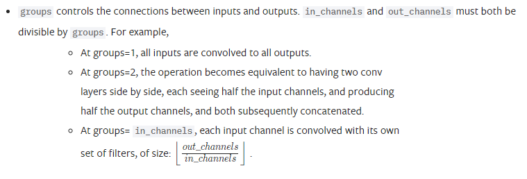
也就是将输入的fetures分为群组，然后分别对每个群组卷积然后连接(cat)到一起，in_channels和out_channels必须同时被groups整除
e.g.输入ci=32, 输出co=32，g=2
那么将输入分为2组，ci1=ci2=ci/g=16, 每组需要的卷积个数为ck1=ck2=co/g=16
ck1ci1=co1=16, ck2ci2=co2=16, concate则最后的输出即为co=32
但是，g=1时计算量为-输入特征层(32)*卷积核的个数（32）,这么多个参数
而g=2时，计算量为-输入特征层(16)*卷积个数(16)*组数(2)

• 当in_channel=groups，卷积就变成了所谓的depthwise convolution
  此时的计算量为1* 1 *32，如果输入输出的feature一样的话

---

• depthwise separable convolutions
  深度可分离卷积

factorized convolutions which factorize a standard convolution into a depthwise convolution and a 1x1 convolution called a pointwise convolution
所谓深度可分离卷积就是一种因式分解卷积的形式，将标准卷积分解为depthwise convolution和pointwise convolution

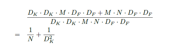
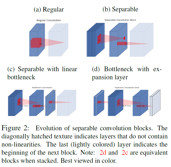
• 实现过程和参数量
  
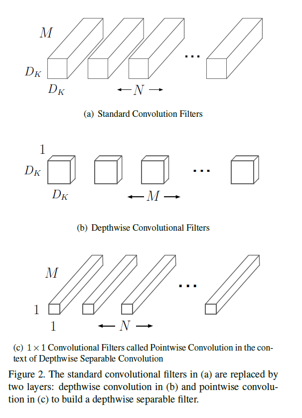
  论文里面的图，大概就是说N个MDkDk的卷积可以分解为b)M个1 * Dk * Dk的卷积和c)N个M * 1 * 1的卷积两步卷积
  这样，参数量就变为原来的好多分之一
  
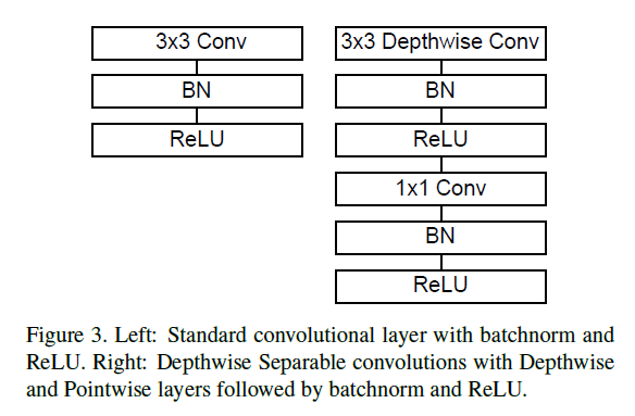
• BN和激活函数
  

---

• Inception models
  具体得查看文献

---

• 使用1x1卷积

This can be implemented with highly optimized general matrix multiply (GEMM) functions. Often convolutions are implemented by a GEMM but require an initial reordering in memory called im2col in order to map it to a GEMM.

实现时，1x1的卷积计算时有优化，可以节省计算时间

---

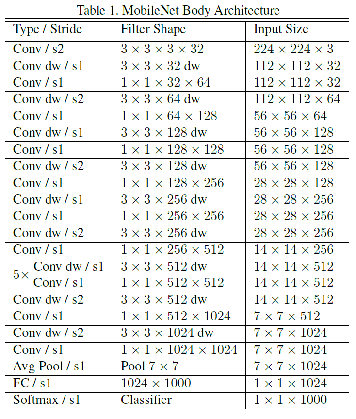
• 网络结构
  

---

以上通过depthwise separable convolutions实现了在损失一点精度的同时大大减少了计算量，那么问题来了

Although the base MobileNet architecture is already small and low latency, many times a specific use case or application may require the model to be smaller and faster.

我们还想要smaller and faster怎么办？文章提出了一种思想，如下

• global hyperparameters trade off latency and accuracy

improve accuracy are not necessarily making networks more efficient with respect to size and speed

这个latency指的是？

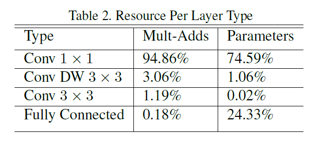
1. FLOPs（具体计算？）== Mult-Adds
   s应该小写，指的是计算量，指的是网络所有操作进行加法和乘法的操作数，但是实际上并不能代表实际操作的运算速度，即使是单独测试每种操作在实际硬件上的耗时也会有偏差，因为不同操作之间的组合也会有耗时
2. 硬件实现耗时

• 超参
  width multiplier and resolution multiplier
  宽度倍率，即feature的通道数；分辨率倍率，指的是输入图像的分辨率

Many different approaches can be generally categorized into either compressing pretrained networks or
training small networks directly. This paper proposes a class of network architectures that allows a model developer to specifically choose a small network that matches the resource restrictions (latency, size) for their application
提供了一类网络可以根据你的应用匹配你的资源限制，例如延时和大小，很吸引人的点

---

他是怎样实现的呢？
也就是在baseline的基础上，width multiplier

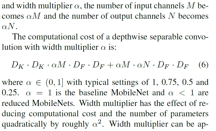
这不是我们想到的基本思想。。。。
resolution multiplier

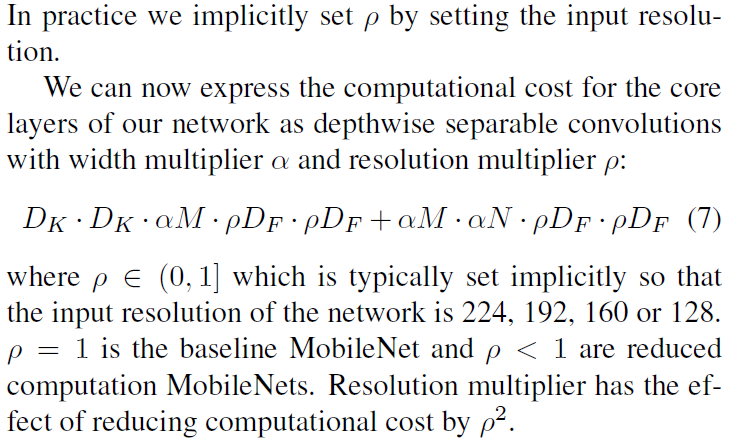
无力吐槽，但是正是由于他们对这个问题有这样一个思考，才有他能想到efficientNet的grid search方法寻找最优dwr的scale， 任何一个简单的思考都是有价值的
下面一个实验蛮有意思的：Narrow vs Shallow

---

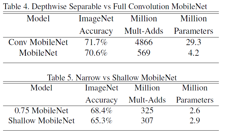
• mobileNetv1总结

1. 使用depthwise separable convolutions其中的1x1的卷积减少了计算量,以及这样一个dw操作中BN和ReLu等操作的使用
2. 对网络的宽度(w),深度(d)和分辨率®有了一点思考，后面的实验说明同样的计算量，可能宽度要优先于深度，存疑

---

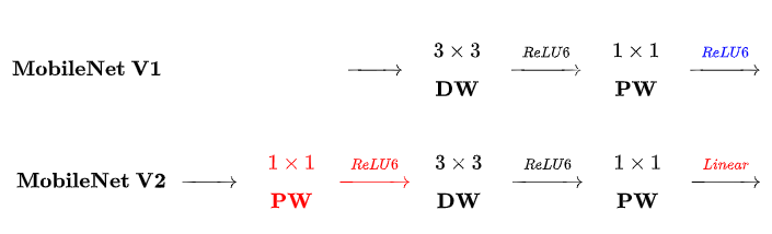
mobileNetv2

文章名字就叫MobileNetV2: Inverted Residuals and Linear Bottlenecks
那么重点肯定就是Inverted Residuals 和 Linear Bottlenecks
反残差和线性瓶颈，不知所云啊，看文章

---

Our main contribution is a novel layer module: the inverted residual with linear bottleneck

• depthwise separable convolutions
  首先v2沿用了这种好用的结构

---

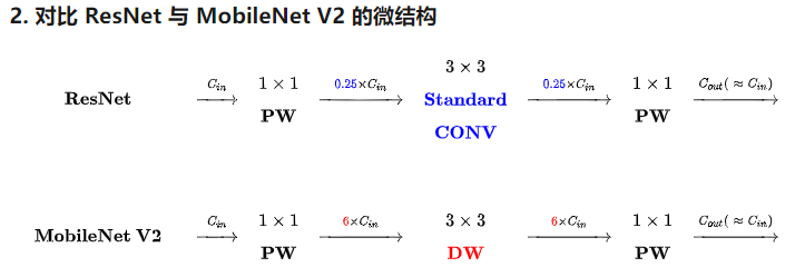
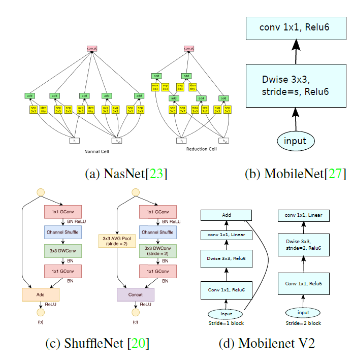
• inverted residuals
  借鉴了ResNet结构，提出反残差结构
  

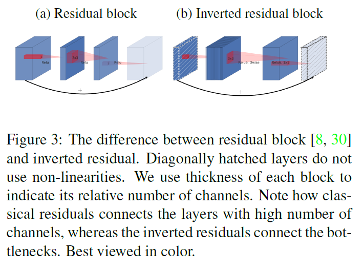
1. 和resnet一样使用shortcuts的连接
2. 但是在前后1x1卷积的时候扩充了卷积通道，故称之为inverted residual

---

• Linear Bottlenecks
  考虑ReLu激活函数在低维空间会导致信息大量缺失，所以最后一层改为线性激活函数
  证明？
  看原文3.2 Linear Bottlenecks
  他认为所谓的manifold of interest，可以embedded到一个低维的子空间
  我们可以通过width multiplier降低这个维度空间
  然而，当我们的神经网络拥有非线性操作后
  他做了一个实验
  
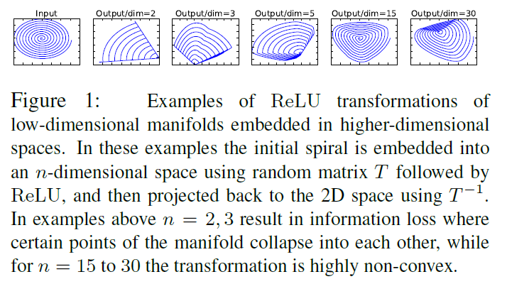
  以上实验用一个随机变换T将输入，就是那个圈圈，变换成高维，再通过ReLu激活，然后再通过T‘变回原来维度，他证明维度越高这种信息的丢失就越少
  神经网络最开始发明ReLu的时候就告诉大家，这个激活函数能够更加突出被激活的神经元，文章都说他更有效了，现在又说他对信息的丢失太严重了，ReLu太难了，当然这个实验并不是要说明这点，ReLu必然会导致信息的稀疏，但他的初衷是去除冗余，但是在这里是为了说明，低维时每一维都具有有效的信息，但是ReLu可能会将他们丢弃了
  
  这里首先将1x1卷积后的激活函数变为线性激活，就是没有激活函数

---

借知乎别人的图说明以上两点


好像文章结构就到这里了
直观看v2的参数比v1不是应该多好多？多了1x1卷积，后面的conv卷积通道还多了好几倍。。。。，还有shortcuts呢？
看看后面怎么圆。。。。

nature of our networks allows us to utilize much smaller input and output dimensions

---

• expansion rate
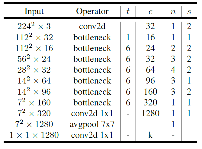
  也就是上面的t，文章为什么使用了常数？

In our experiments we find that expansion rates between 5 and 10 result in nearly identical performance curves, with smaller networks being better off with slightly smaller expansion rates and larger networks having slightly better performance with larger expansion rates.

因为实验证明过大带来的性能影响微乎其微

---

• width multiplier

width multipliers of 0:35 to 1:4

---

• 文章各网络结构
  
  文章MobileNetv1，v2都看过了，shuffleNet待看，NasNet再说吧
  最后好像还有证明，有机会再看一遍

---

DARTS那套东西最终还是没有看。。。。
最近一直在做matting，发现基础奇缺，分割的框架大概看了下deeplabv3plus的网络设计使用mv2为backbone，但是更小的网络怎样设计和训练呢？到现在我还是曾经的那个少年—一无所知，所以我连尝试的方向都没有。几周前，lee推荐了GAN Compress和once for all，听起来是一个解决方案，静下心来好好看文章和代码，或许会有很多收获

---

ONCE FOR ALL - OFA

• abstract

1. Conventional approaches either manually design or use neural architecture search (NAS) to find a specialized
   neural network and train it from scratch for each case, which is computationally prohibitive (causing CO2 emission as much as 5 cars’ lifetime Strubell et al. (2019)) thus unscalable

• 确实每个特定的网络，不管是人工设计或者NAS搜索都需要从头开始训练
• CO2这个说法真有点意思2333

---

• introduction

repeat the network design process and retrain the designed network from scratch for each case

we decouple the model training stage and the neural architecture search stage

以前的网络设计需要repeat设计和retrain
现在解耦了模型训练和模型设计，只需要all里面取出subnetwork，不用retrain

---

In the model specialization stage, we sample a subset of sub-networks to train an accuracy predictor and latency predictors. Given the target hardware and constraint, a predictor-guided architecture search (Liu et al., 2018) is conducted to get a specialized sub-network, and the cost is negligible

• 这里怎么做的? 这两个predictors怎么train

---

• problem formalization
  
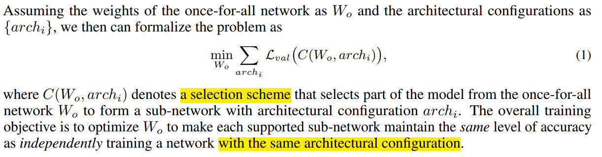
  same architectural configuration指的是？

---

• Architecture Space

architectures	spaces
resolution	128:224:4
depth	{2, 3, 4}
width expansion ratio	{3, 4 ,6}
kernel size	{3, 5, 7}

一个unit = $((3\times 3{)}^2+(3\times 3{)}^3+(3\times 3{)}^4=7371$
如果有5个unit就是 $7371^5=21,758,655,492,572,485,851$这么多结构。。。。无语凝噎

---

• train
• naive approach

1. 将OFA看作一个multi-objective problem,每一个objective都是一个subnet，然后联合优化就像上面的公式1一样，但是这样要联合优化$2\times 10^{19}$个subnet，计算量和硬件都吃不消
2. 另外就是从如此多的subnet中sample一些更新 in each update，但是这样由于参数共享带来的干扰，实验发现会有较大的精度下降

---

• progressive shrinking (PS)
  首先训练一个full-net，然后再每个纬度逐步fine-tune

---

下面我们来看看每个维度调优的过程

---

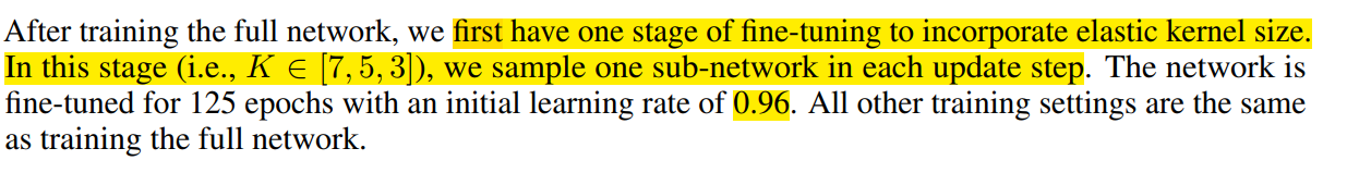
• kernel size

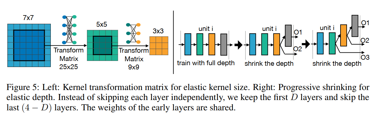
1. 训练完fullnet后，先优化kernel size，这是一个one-stage的优化过程，每次更新选择一个subnet每层随机选择一个k更新网络

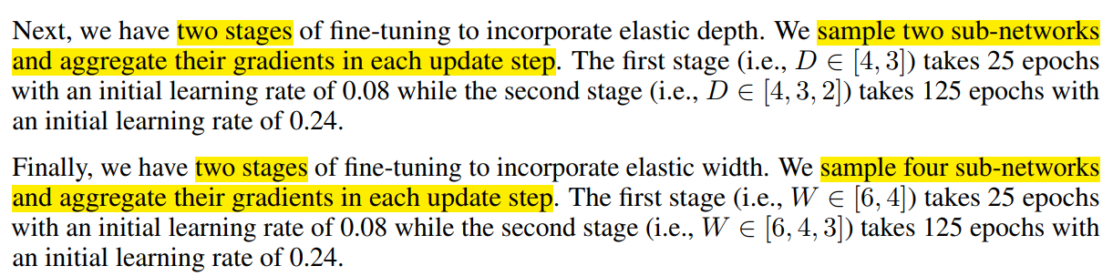
• Depth

2. 再优化D，这是一个two-stage的过程，第一步随机选择[4, 3],再随机选择[4,3,2]，每次更新选择两个subnet联合更新网络，这个参数是每个layer重复堆叠的次数

• Width

3. 最后优化宽度，也是一个two-stage的过程，第一步随机选择[6,4]，再随机选择[6,4,3],每次更新选择四个subnet联合更新网络，这个参数是每个layer中channel的膨胀系数，即channel在原始channel的基础上扩充多少倍

---

• predictor
  训练一个预测器选择subnet，说实话我没怎么看懂这个部分
  
  大概意思是，选择不同的参数配置，每个参数配置对应一个机器的延时，相当于回归？

---

• 代码后面再看，先看一个GAN compress的文章

---

GAN Compress

没有那么仔细看，随便翻了一下
文章最后的消融实验证明

• Effectiveness of convolution decomposition
  separable conv更有效，在downsample阶段
  看一看代码吧

---

重新阅读一下GAN Compression

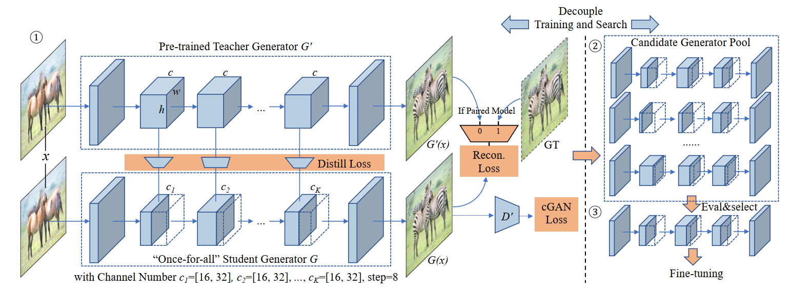
• Abstract
  使用GAN Compression 可以使得cGANs 模型例如pix2pix, CycleGan 和GauGAN 压缩9-21倍
  从两个方面考虑问题

1. First, to stabilize the GAN training, we transfer knowledge of multiple intermediate representations of the original model to its compressed model, and unify unpaired and paired learning
   为了稳定GAN的训练使用transfer learning

2. Second, instead of reusing existing CNN designs, our method automatically finds efficient architectures via neural architecture search (NAS). To accelerate the search process, we decouple the model training and architecture search via weight sharing
   使用NAS搜索合适的网络架构，为了加速搜索，使用权值共享