斯坦福课程导论(CS231n)：Image Classification: Data-driven Approach, k-Nearest Neighbor, train/val/test split

本文是一篇针对非计算机视觉领域群众的导论性的文章，介绍其中的图像分类问题和相应的数据驱动方法。文章目录结构如下：

图像分类

驱动：本节介绍在将输入图像划分至预设的分类集合中某项类别中，所遇到的一些问题。尽管它在计算机视觉中很简单，但仍然是其中的核心问题之一，具有各式各样的应用。此外，在往后的课程中，很多看似不同的计算机视觉任务（如物体识别，分割）都可以被列为图像分类。
案例：假如，将下图通过图像分类模型，匹配将其划分至四类标签{cat,dog,hat,mug}，并计算出各类的相似概率。计算机认为下图是一个大型的三维数据。例如，图片大小为248 x400，包含RGB三个波段，那其相当于包含248 x 400 x 3 个像素点，共计297,600个。每个像素点值域为0~255，0代表黑色，255代表白色。我们的任务是将这个百万个像素点划分为统一的一个标签，例如“cat”。

The task in Image Classification is to predict a single label (or a distribution over labels as shown here to indicate our confidence) for a given image. Images are 3-dimensional arrays of integers from 0 to 255, of size Width x Height x 3. The 3 represents the three color channels Red, Green, Blue.

---

挑战：由于图片识别是与人相关的行为操作，但他需要从计算机视觉算法的角度思考问题。大体罗列下遇到的问题：

• 视角变量。同个物体可在不同的角度下拍摄，图片结果截然不同。
• 尺度变量。物体具有大小的物理含义。
• 变形。物体拍摄的变形因素。
• 吸收变量。物体的兴趣区域可能被隐藏。一些时候只有少量的兴趣区域被展示出来（少至几个像素）
• 照明变量。拍摄的光照条件影像像素结果的亮度值。
• 背景干扰。物体被相似的背景信息干扰，影响判别。
• 内部差异。物体内部可包含更细的子物体，各子物体不尽相同。

一个好的图像分类模型必须对上述的变量具有不变性，同时能灵敏区分物体内部的差异因素。

---

数据驱动方法：编写一个怎样的算才能将图像分类至特定的类别呢？显然，诸如对像素数据的排序这些方式，并不能做到。因此，在尝试通过编码的方式对每种特定类型进行特殊定义之外，本文采用的方法是与一个你会带一个孩子：我们将向计算机输入样例类别的图片数据，开发出一种计算机学习的算法使计算机学习各类类别的数据特征。这种方法即称为数据驱动的方式，因为它依赖于对分类图像数据的学习。如下是一个分类集合的例子：

---

An example training set for four visual categories. In practice we may have thousands of categories and hundreds of thousands of images for each category.

---

图像分类管线：我们了解到图像分类在将一堆代表图像信息的像素值数组识别一个特定的类别。其整个任务的流程如下所示：
- 输入。数据输入包括N幅已经分类好的影像，分类类别达K种。我们称之为训练样本。
- 学习。我们的任务是通过训练样本学习各类图像的特征信息。这部我们称之为样本训练，或者模型学习。
- 预测。最后，我们通过对新数据的分类识别来评估分类模型的质量。比较图像真实的分类信息和预测的分类信息。当然，我们希望预测结果与真实情况（我们称之为the ground truth）相符。

最邻近分类器

我们第一个方法，采用最邻近分类器。这个分类器与卷积神经网络无关且不常用，但它能给我们一个对图像分类问题基本方法的一些灵感。
样例的分类数据集:CIFAR-10。一个著名的图像分类数据集便是CIFAR-10。它有 60,000个32x32的小图像组成，每个图像被标记为10个固定类别(如”airplane, automobile, bird,等”)中的一个。这60,000个图像其中50,000 被划分为训练集，另外10,000 被划分为测试集。下图随机从10类中挑选样本图片。

---

Left: Example images from the CIFAR-10 dataset. Right: first column shows a few test images and next to each we show the top 10 nearest neighbors in the training set according to pixel-wise difference.

---

假设当前我们有50,000 个已经分类的CIFAR-10训练集数据，需要利用他们对剩余的10,000个数据进行分类。最邻近分类器针对每一幅测试图片，会去训练集数据中一一比对，从而预报处最接近的一张训练图片。在上图右侧中，我们可以看到10张测试图分别找到几张最邻近图片。结果发现，10个测试图片中仅3幅比对到了正确的类别。例如，第八行中最邻近的训练图片是一幅红色的轿车，与真实的马类别不符，这种情况可能是强背景导致的结果。因此，马的图像在本例中被错认为一辆轿车。

大家可能思考我们如何比对两张图的方式，实际上它们只是 32 x 32 x 3的矩阵而已。其中一种最简单的方式，就是一一对比每个像素值的差异，最后将其结果相加得到。换而言之，给予两幅图像，其矢量表示为 I1,I2，一个可行的比较方法可以是L1 distance:

$$d1(I1,I2)=∑p|Ip1−Ip2|$$
其中数据集合就是如此，以下是该公式的图形化表示:

---

An example of using pixel-wise differences to compare two images with L1 distance (for one color channel in this example). Two images are subtracted elementwise and then all differences are added up to a single number. If two images are identical the result will be zero. But if the images are very different the result will be large.

---

后面引申出了最邻近的K个值的算法，从最邻近的一个分类扩展为K个分类。
与此同时，对K这个参数的选择成为一个问题（K值为多少时，分类效果最好），于是就是超参数调参方法，即Hyperparameter tuning。
tuning的过程有很多问题会出现，需要考虑：过拟合、欠拟合等。
同时，有几个关键的要点需要牢记：

Evaluate on the test set only a single time, at the very end.(测试集数据只能在最后的最后使用，最后测试识别效果的，调参的时候不能介入)
Split your training set into training set and a validation set. Use validation set to tune all hyperparameters. At the end run a single time on the test set and report performance.(把训练集数据划分为训练集和验证集数据。使用验证集数据进行调参。最后，采用测试集数据进行测试，导出性能报告)
提供了两种方法：最简单的一种，及将原先的训练样本集再分割为两部分，一部分为训练集，一部分为验证集，先训练后验证，调参。另一种（Cross-validation），将训练样本均分为若干部分，其中一部分为验证集，其余的都为训练集，然后训练验证，之后再选取另一部分为验证集，其余为训练集，进行训练验证。如此循环，最后平均化所有的验证精度，从而再确定调参。

---

Example of a 5-fold cross-validation run for the parameter k. For each value of k we train on 4 folds and evaluate on the 5th. Hence, for each k we receive 5 accuracies on the validation fold (accuracy is the y-axis, each result is a point). The trend line is drawn through the average of the results for each k and the error bars indicate the standard deviation. Note that in this particular case, the cross-validation suggests that a value of about k = 7 works best on this particular dataset (corresponding to the peak in the plot). If we used more than 5 folds, we might expect to see a smoother (i.e. less noisy) curve.

---

实际操作中，如果样本数据多的话，可以直接使用第一种方法，如果样本少的话，需要使用第二种方法，可将样本集合均分为3、5、10类等等。

---

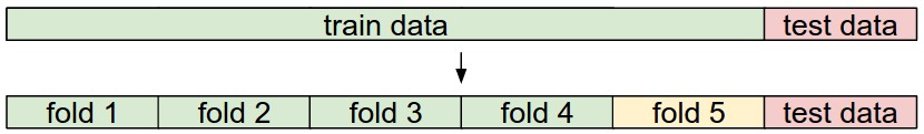
Common data splits. A training and test set is given. The training set is split into folds (for example 5 folds here). The folds 1-4 become the training set. One fold (e.g. fold 5 here in yellow) is denoted as the Validation fold and is used to tune the hyperparameters. Cross-validation goes a step further iterates over the choice of which fold is the validation fold, separately from 1-5. This would be referred to as 5-fold cross-validation. In the very end once the model is trained and all the best hyperparameters were determined, the model is evaluated a single time on the test data (red).

---

最邻近分类器的优缺点

优点：
- 算法简单可实现
- 不用训练（只要图片数据有就行，不需要生成训练的一些结果）
缺点：
- 测试时花费计算时间（需要对每个图片进行一一比对，很耗时。这个问题很重要，大家对训练时间的长短并不介意，但对测试的时间很在意）
事实上，深度神经网络后面发展了，将这个测试的代价转移到另外的极端方向：训练代价极其昂贵，而一旦训练完毕，测试非常快速简单。这种方式更适应于实际应用。

另外，最邻近分类法的计算复杂度也是一个常见的研究方向，并已经开发出了一些近似最邻近（ANN）算法和库，来加速最邻近查找方法 (e.g. FLANN)。这些算法权衡了最近李。。。。

最邻近分类法子在某些情况下是个不错的分类选择（尤其是数据为低纬度的），但是它一般较少应用于实际的图像分类应用中。一个问题是图像是高纬度物体，包含很多像素值，且高纬度空间的距离很特殊。下图就表示虽然图片仅是镂空部分或者变暗了一些，它与原图的匹配相似度很低（pixel-wise距离），说明上述方法并不能用于知觉或语义相似度。

---

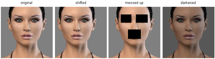
Pixel-based distances on high-dimensional data (and images especially) can be very unintuitive. An original image (left) and three other images next to it that are all equally far away from it based on L2 pixel distance. Clearly, the pixel-wise distance does not correspond at all to perceptual or semantic similarity.

---

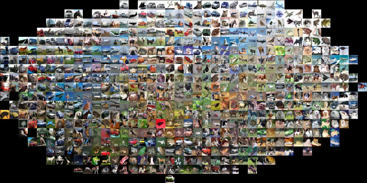
以下的图像告诉我们像素点的差异是无法完全比对影像成功的。采用一种可视化技术t-SNE将CIFAR-10的图片结合起来，将其嵌入二维坐标系，从而使得 (local) pairwise distances达到最适应。在此可视化中，在附近的图像会很接近原始图像，依照上述提出的L2 pixelwise distance 公式。

---

(http://cs231n.github.io/assets/pixels_embed_cifar10.jpg)

CIFAR-10 images embedded in two dimensions with t-SNE. Images that are nearby on this image are considered to be close based on the L2 pixel distance. Notice the strong effect of background rather than semantic class differences. Click here for a bigger version of this visualization.

---

尤其，。。。。。

结论

• We introduced the problem of Image Classification, in which we are given a set of images that are all labeled with a single category.
• We are then asked to predict these categories for a novel set of test images and measure the accuracy of the predictions.
• We introduced a simple classifier called the Nearest Neighbor classifier. We saw that there are multiple hyper-parameters (such as value of k, or the type of distance used to compare examples) that are associated with this classifier and that there was no obvious way of choosing them.
• We saw that the correct way to set these hyperparameters is to split your training data into two: a training set and a fake test set, which we call validation set. We try different hyperparameter values and keep the values that lead to the best performance on the validation set.
• If the lack of training data is a concern, we discussed a procedure called cross-validation, which can help reduce noise in estimating which hyperparameters work best.
• Once the best hyperparameters are found, we fix them and perform a single evaluation on the actual test set.
• We saw that Nearest Neighbor can get us about 40% accuracy on CIFAR-10. It is simple to implement but requires us to store the entire training set and it is expensive to evaluate on a test image.

In next lectures we will embark on addressing these challenges and eventually arrive at solutions that give 90% accuracies, allow us to completely discard the training set once learning is complete, and they will allow us to evaluate a test image in less than a millisecond.

Summary: Applying kNN in practice

If you wish to apply kNN in practice (hopefully not on images, or perhaps as only a baseline) proceed as follows:

Preprocess your data: Normalize the features in your data (e.g. one pixel in images) to have zero mean and unit variance. We will cover this in more detail in later sections, and chose not to cover data normalization in this section because pixels in images are usually homogeneous and do not exhibit widely different distributions, alleviating the need for data normalization.
If your data is very high-dimensional, consider using a dimensionality reduction technique such as PCA (wiki ref, CS229ref, blog ref) or even Random Projections.
Split your training data randomly into train/val splits. As a rule of thumb, between 70-90% of your data usually goes to the train split. This setting depends on how many hyperparameters you have and how much of an influence you expect them to have. If there are many hyperparameters to estimate, you should err on the side of having larger validation set to estimate them effectively. If you are concerned about the size of your validation data, it is best to split the training data into folds and perform cross-validation. If you can afford the computational budget it is always safer to go with cross-validation (the more folds the better, but more expensive).
Train and evaluate the kNN classifier on the validation data (for all folds, if doing cross-validation) for many choices of k (e.g. the more the better) and across different distance types (L1 and L2 are good candidates)
If your kNN classifier is running too long, consider using an Approximate Nearest Neighbor library (e.g. FLANN) to accelerate the retrieval (at cost of some accuracy).
Take note of the hyperparameters that gave the best results. There is a question of whether you should use the full training set with the best hyperparameters, since the optimal hyperparameters might change if you were to fold the validation data into your training set (since the size of the data would be larger). In practice it is cleaner to not use the validation data in the final classifier and consider it to be burned on estimating the hyperparameters. Evaluate the best model on the test set. Report the test set accuracy and declare the result to be the performance of the kNN classifier on your data.

Further Reading

Here are some (optional) links you may find interesting for further reading:

A Few Useful Things to Know about Machine Learning, where especially section 6 is related but the whole paper is a warmly recommended reading.
Recognizing and Learning Object Categories, a short course of object categorization at ICCV 2005.