【无线传感网】LEACH路由算法

原创已于 2025-08-21 15:32:00 修改 · 2.4w 阅读

7 ·

CC 4.0 BY-SA版权

文章标签：

#人工智能 #机器学习 #网络 #matlab #物联网

于 2024-06-16 23:01:16 首次发布

无线传感网专栏收录该内容

13 篇文章

订阅专栏

5、LEACH路由算法matlab代码解析

源代码下载：https://download.youkuaiyun.com/download/xiaoyingxixi1989/86911140?spm=1003.2166.3001.6637.8

1、LEACH路由算法简介

LEACH协议，全称是“低功耗自适应集簇分层型协议” (Low Energy Adaptive Clustering Hierarchy)，是一种无线传感器网络路由协议。基于LEACH协议的算法，称为LEACH算法。

2、LEACH路由算法的基本思想

LEACH路由协议与以往的路由协议的不同之处在于其改变了以往簇头是固定的概念，以循环的方式随机选择簇头节点，将整个网络的能量负载平均分配到每个传感器节点中，从而达到降低网络能源消耗、提高网络整体生存时间的目的。仿真表明，与一般的平面多跳路由协议和静态分层算法相比，LEACH分簇协议可以将网络生命周期延长15%。

3、LEACH路由算法的数学模型

在实际操作时使用了“轮”（Rounds）的概念，它的执行过程是按照一定周期性的。每一轮可以分为成簇阶段和数据传输阶段

3.1 成阶段

每一个无线传感器网络节点随机生成［0，1］的随机数，通过公式（1）的阈值判定公式产生一个阈值，将随机值和阈值进行比较，如果这个随机值小于阈值 T(n) ，则成为簇头节点。T(n)按公式（2.1）计算：

其中,r为目前选举轮数，p为簇头节点所占百分数，G 为最近1/p轮没有成为簇头的节点集合。从公式(2.1)可以知道，其中随着轮数的增加，T(n)的值也逐渐增大，此刻的阈值越大未担任过簇头的节点在下一轮中成为簇头的概率越大。

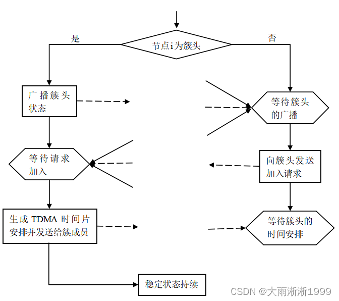
当选簇头广播簇头消息，非簇头节点根据接收信号的强度，选择强度最大的加入该簇。簇头节点采用时分多址（TDMA）方式安排时间间隙。

3.2 簇的数据传输阶段

进入数据传输阶段后，非簇头节点根据时间间隙向其簇头发送数据，然后进入睡眠状态，等待下一个时间间隙。簇头节点将接收到的数据进行融合，然后发送到汇聚节点。持续一定的时间后，进行新一轮的分簇阶段。成簇流程图如下

4、LEACH路由算法的优缺点

4.1 LEACH 协议优点

（1）采用随机选举簇头，使网络中节点能够交替成为簇头，避免一直充当簇头节点而使能量快速消耗；

（2）在数据传输阶段采用了数据融合，减少了不必要的能量消耗。

4.2 LEACH 协议缺点

(1)由于簇头选择比较随机，部分能量较低的节点可能成为簇头节点，这样簇头节点由于能量很低，可能在数据传输过程中能量耗尽，这样可能造成接收数据的不完整性；

(2) 簇头节点直接与汇聚节点进行通信通信，距离汇聚节点较远的节点消耗的能量将大大增加，导致这部分节点能耗较大，使远离汇聚节点的节点能量过早耗尽，造成网络监测的盲区。

5、LEACH路由算法matlab代码解析

%function EE=Leach()
function [DEAD]=Leach()
%Field Dimensions - x and y maximum (in meters)
xm=200;                                   %定义X与Y区域
ym=200;

%x and y Coordinates of the Sink
sink.x=0.5*xm;                            %sink节点位置
sink.y=1.75*ym;

%Number of Nodes in the field
n=100;                                     %节点总数

%Optimal Election Probability of a node to become cluster head
p=0.1;                                    %簇头比例

%Initial Energy 
Eo=0.5;                                   %初始能量
%Eelec=Etx=Erx
ETX=50*0.000000001;                       %节点发送数据能耗
ERX=50*0.000000001;                       %节点接收数据能耗
%Transmit Amplifier types
Efs=10*0.000000000001;
Emp=0.0013*0.000000000001;
%Data Aggregation Energy
EDA=5*0.000000001;                         %聚集数据包能耗

 
%maximum number of rounds
rmax=2000;                                 %最大轮数

 

%Computation of do
do=sqrt(Efs/Emp);                          %计算do

%Creation of the random Sensor Network
figure(1);
for i=1:1:n
    S(i).xd=rand(1,1)*xm;                  %随机节点的X轴坐标    
    XR(i)=S(i).xd;
    S(i).yd=rand(1,1)*ym;                  %随机节点Y轴位置
    YR(i)=S(i).yd;
    S(i).E=Eo;                             %初始化节点能量均为1
    S(i).G=0;
    %initially there are no cluster heads only nodes
    S(i).type='N';                         %初始化节点，全部为普通节点
    plot(S(i).xd,S(i).yd,'o');
    hold on;
end

S(n+1).xd=sink.x;                          %初始化sink节点位置
S(n+1).yd=sink.y;
plot(S(n+1).xd,S(n+1).yd,'x');
    
        
%First Iteration
figure(1);

%counter for CHs
countCHs=0;
%counter for CHs per round
rcountCHs=0;
%cluster=0;

countCHs;
rcountCHs=rcountCHs+countCHs;
flag_first_dead=0;

for r=0:1:rmax
    r

  %Operation for epoch

  if(mod(r, round(1/p) )==0)
    for i=1:1:n
        S(i).G=0;
        S(i).cl=0;
    end
  end

  hold off;

  %Number of dead nodes
  dead=0;                        %死亡节点数
 

  %counter for bit transmitted to Bases Station and to Cluster Heads
  packets_TO_BS=0;
  packets_TO_CH=0;
  %counter for bit transmitted to Bases Station and to Cluster Heads per round
  PACKETS_TO_CH(r+1)=0;
  PACKETS_TO_BS(r+1)=0;

  figure(1);
  
 

  for i=1:1:n
    %checking if there is a dead node
    if (S(i).E<=0)                              %辨别死亡节点
        plot(S(i).xd,S(i).yd,'red .');
        dead=dead+1;
        hold on;    
    end
    if (S(i).E>0)
        S(i).type='N';
        plot(S(i).xd,S(i).yd,'o');
        hold on;
    end
  end
  plot(S(n+1).xd,S(n+1).yd,'x');


  STATISTICS(r+1).DEAD=dead;
  DEAD(r+1)=dead;
 
  %When the first node dies
  if (dead==1)
    if(flag_first_dead==0)
        first_dead=r
        flag_first_dead=1;
    end
  end

  countCHs=0;
  cluster=1;
  for i=1:1:n
   if(S(i).E>0)
   temp_rand=rand;     
     if ( (S(i).G)<=0)

      %Election of Cluster Heads
       if(temp_rand<= (p/(1-p*mod(r,round(1/p)))))
            countCHs=countCHs+1;
            packets_TO_BS=packets_TO_BS+1;
            PACKETS_TO_BS(r+1)=packets_TO_BS;
            
            S(i).type='C';
            S(i).G=round(1/p)-1;
            C(cluster).xd=S(i).xd;
            C(cluster).yd=S(i).yd;
            plot(S(i).xd,S(i).yd,'k*');
            
            distance=sqrt( (S(i).xd-(S(n+1).xd) )^2 + (S(i).yd-(S(n+1).yd) )^2 );
            C(cluster).distance=distance;
            C(cluster).id=i;
            X(cluster)=S(i).xd;
            Y(cluster)=S(i).yd;
            cluster=cluster+1;
            
            %Calculation of Energy dissipated
            distance;
            if (distance>do)
                S(i).E=S(i).E- ( (ETX+EDA)*(4000) + Emp*4000*( distance*distance*distance*distance )); 
            end
            if (distance<=do)
                S(i).E=S(i).E- ( (ETX+EDA)*(4000)  + Efs*4000*( distance * distance )); 
            end
       end     
    
     end
   end 
 end

STATISTICS(r+1).CLUSTERHEADS=cluster-1;
CLUSTERHS(r+1)=cluster-1;

%Election of Associated Cluster Head for Normal Nodes
for i=1:1:n
   if ( S(i).type=='N' && S(i).E>0 )
     if(cluster-1>=1)
       min_dis=sqrt( (S(i).xd-S(n+1).xd)^2 + (S(i).yd-S(n+1).yd)^2 );
       min_dis_cluster=1;
       for c=1:1:cluster-1
           temp=min(min_dis,sqrt( (S(i).xd-C(c).xd)^2 + (S(i).yd-C(c).yd)^2 ) );
           if ( temp<min_dis )
               min_dis=temp;
               min_dis_cluster=c;
           end
       end
       
       %Energy dissipated by associated Cluster Head
            min_dis;
            if (min_dis>do)
                S(i).E=S(i).E- ( ETX*(4000) + Emp*4000*( min_dis * min_dis * min_dis * min_dis)); 
            end
            if (min_dis<=do)
                S(i).E=S(i).E- ( ETX*(4000) + Efs*4000*( min_dis * min_dis)); 
            end
        %Energy dissipated
        if(min_dis>0)
          S(C(min_dis_cluster).id).E = S(C(min_dis_cluster).id).E- ( (ERX + EDA)*4000 ); 
         PACKETS_TO_CH(r+1)=n-dead-cluster+1; 
        end

       S(i).min_dis=min_dis;
       S(i).min_dis_cluster=min_dis_cluster;
           
   end
 end
end
hold on;

countCHs;
rcountCHs=rcountCHs+countCHs;



%Code for Voronoi Cells Unfortynately if there is a small number of cells, Matlab's voronoi procedure has some problems

[vx,vy]=voronoi(X,Y);
plot(X,Y,'r*',vx,vy,'b-');
 hold on;
 voronoi(X,Y);
 axis([0 xm 0 ym]);
E=0;
for j=1:1:n
   
   E=E+S(i).E;
end
EE(r+1)=E*0.01;
end
 
%figure(2);
%hold off;
%plot(EE,'+');
%legend('leach',1);

%%%%%%%%%%%%%%%%%%%%%%%%%%%%%%%%%%%   STATISTICS    %%%%%%%%%%%%%%%%%%%%%%%%%%%%%%%%%%%
%                                                                                     %
%  DEAD  : a rmax x 1 array of number of dead nodes/round 
%  DEAD_A : a rmax x 1 array of number of dead Advanced nodes/round
%  DEAD_N : a rmax x 1 array of number of dead Normal nodes/round
%  CLUSTERHS : a rmax x 1 array of number of Cluster Heads/round
%  PACKETS_TO_BS : a rmax x 1 array of number packets send to Base Station/round
%  PACKETS_TO_CH : a rmax x 1 array of number of packets send to ClusterHeads/round
%  first_dead: the round where the first node died                   
%                                                                                     %
%%%%%%%%%%%%%%%%%%%%%%%%%%%%%%%%%%%%%%%%%%%%%%%%%%%%%%%%%%%%%%%%%%%%%%%%%%%%%%%%%%%%%%%