


模型选择
训练误差和泛化误差
训练误差:模型在训练数据上的误差
泛化误差:模型在新数据上的误差
举个例子:根据例子:根据摸考成绩来预测未来考试分数
- 在过去的考试中表现很好(训练误差)不代表未来考试一定会好(泛化误差)
- 学生 A 通过背书在摸考中拿到很好成绩
- 学生 B 知道答案后面的原因
验证数据集和测试数据集
- 验证数据集:一个用来评估模型好坏的数据集
- 例如拿出 50% 的训练数据
- 不要跟训练数据混在一起(常犯错误)
- 测试数据集:只用一次的数据集。例如
- 未来的考试
- 我出价的房子的实际成交价
- 用在 Kaggle 私有排行榜中的数据集
K - 则交叉验证
- 在没有足够多数据时使用(这是常态)
- 算法:
- 将训练数据分割成K块
- Fori=1,…,K
- 使用第 i 块作为验证数据集,其余的作为训练数据
- 报告K个验证集误差的平均
- 常用:K=5或10
在非大数据集上通常使用 k - 折交叉验证
过拟合和欠拟合
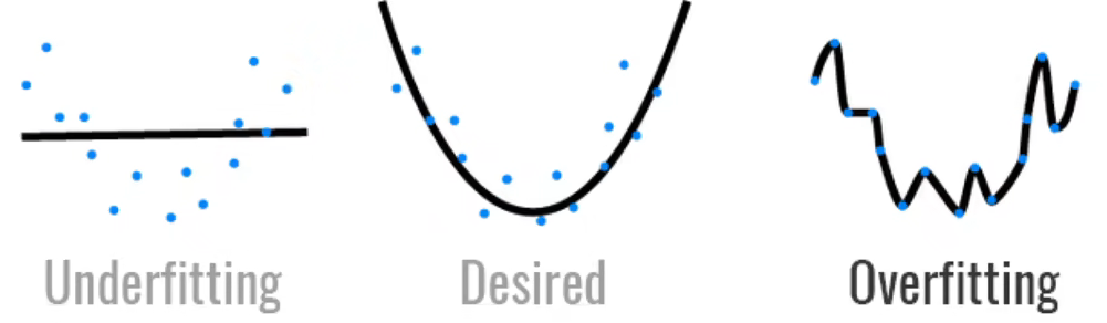
模型容量
- 拟合各种函数的能力
- 低容量的模型难以拟合训练数据
- 高容量的模型可以记住所有的训练数据
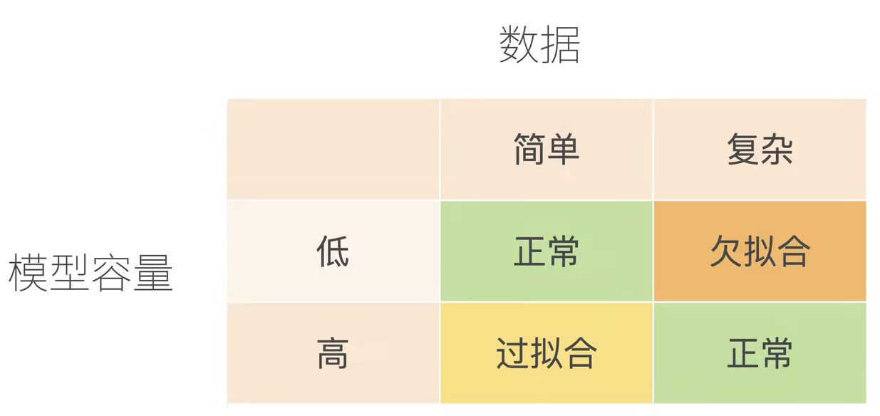
模型容量的影响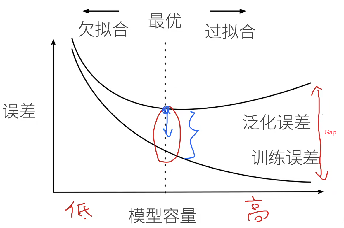
代码
首先导入必要的环境:
import math
import numpy as np
import torch
from torch import nn
from d2l import torch as d2l
接下来构造如下的数据集:
给定
x
x
x,使用以下三阶多项式来生成训练和测试数据的标签:
y
=
5
+
1.2
x
−
3.4
x
2
2
!
+
5.6
x
3
3
!
+
ϵ
where
ϵ
∼
N
(
0
,
0.
1
2
)
.
y = 5 + 1.2x - 3.4\frac{x^2}{2!} + 5.6 \frac{x^3}{3!} + \epsilon \text{ where } \epsilon \sim \mathcal{N}(0, 0.1^2).
y=5+1.2x−3.42!x2+5.63!x3+ϵ where ϵ∼N(0,0.12).
噪声项
ϵ
\epsilon
ϵ服从均值为0且标准差为0.1的正态分布。在优化的过程中,我们通常希望避免非常大的梯度值或损失值。这就是我们将特征从
x
i
x^i
xi调整为
x
i
i
!
\frac{x^i}{i!}
i!xi的原因,这样可以避免很大的
i
i
i带来的特别大的指数值。我们将为训练集和测试集各生成100个样本。
# 定义多项式的最大阶数
max_degree = 20  # 这意味着我们将考虑最高到20次的多项式特征
# 定义训练集和测试集的大小
n_train, n_test = 100, 100  # 每个数据集包含100个样本
# 初始化真实的权重向量
true_w = np.zeros(max_degree)  # 创建一个长度为max_degree的零向量
# 设置多项式的前四个系数的真实值
true_w[0:4] = np.array([5, 1.2, -3.4, 5.6])  # 只有前四个系数是非零的
# 生成特征数据
features = np.random.normal(size=(n_train + n_test, 1))  # 生成正态分布的特征数据
np.random.shuffle(features)  # 打乱这些特征数据的顺序
# 将特征转换为多项式特征
poly_features = np.power(features, np.arange(max_degree).reshape(1, -1))  # 生成从0次到max_degree次的多项式特征
# arange用于生成一个从0到最大值-1的一维数组,得到的是一个只有一行的二维数组
# power计算两个数组对应元素的幂
# 对多项式特征进行标准化(除以阶乘)
for i in range(max_degree):
    poly_features[:, i] /= math.gamma(i + 1)  # i次方的特征除以(i+1)阶乘
    # [:,i]选取第i列的所有数据,这里就只有一个
    # gamma(n) = (n-1)!,这里用来归一化多项式特征
# 生成标签数据
labels = np.dot(poly_features, true_w)  # 通过多项式特征与真实权重的点积来生成标签
labels += np.random.normal(scale=0.1, size=labels.shape)  # 向标签添加一些高斯噪声,模拟现实世界中的误差
下面看一下前两个样本:
# NumPy ndarray转换为tensor
true_w, features, poly_features, labels = [
	torch.tensor(x, dtype = torch.float32)
	for x in [true_w, features, poly_features, labels]]

features[:2], poly_features[:2, :], labels[:2]

下面实现一个函数来评估模型在给定数据集上的损失:
def evaluate_loss(net, data_iter, loss):  #@save
    """评估给定数据集上模型的损失"""
    # 初始化一个 Accumulator 对象,用于累积损失总和和样本数量
    metric = d2l.Accumulator(2)  # 损失的总和, 样本数量
    # 遍历数据迭代器中的每个批次
    for X, y in data_iter:
        # 使用模型进行前向传播,得到预测值
        out = net(X)
        # 将真实标签的形状调整为与预测值相同的形状
        y = y.reshape(out.shape)
        # 计算预测值与真实值之间的损失
        l = loss(out, y)
        # 累加当前批次的损失总和
        metric.add(l.sum(), l.numel())
    # 计算平均损失值
    return metric[0] / metric[1]
下面定义训练函数:
def train(train_features, test_features, train_labels, test_labels,
          num_epochs=400):
    loss = nn.MSELoss(reduction='none')
    input_shape = train_features.shape[-1]
    # 不设置偏置,因为我们已经在多项式中实现了它
    net = nn.Sequential(nn.Linear(input_shape, 1, bias=False)) # 不需要偏置
    batch_size = min(10, train_labels.shape[0])
    train_iter = d2l.load_array((train_features, train_labels.reshape(-1,1)),
                                batch_size)
    test_iter = d2l.load_array((test_features, test_labels.reshape(-1,1)),
                               batch_size, is_train=False)
    trainer = torch.optim.SGD(net.parameters(), lr=0.01)
    animator = d2l.Animator(xlabel='epoch', ylabel='loss', yscale='log',
                            xlim=[1, num_epochs], ylim=[1e-3, 1e2],
                            legend=['train', 'test'])
    for epoch in range(num_epochs):
        d2l.train_epoch_ch3(net, train_iter, loss, trainer)
        if epoch == 0 or (epoch + 1) % 20 == 0:
            animator.add(epoch + 1, (evaluate_loss(net, train_iter, loss),
                                     evaluate_loss(net, test_iter, loss)))
    print('weight:', net[0].weight.data.numpy())
展示正常情况
首先使用三阶多项式函数,它与数据生成函数的阶数相同。结果表明,该模型能有效降低训练损失和测试损失。学习到的模型参数也接近真实值 w = [ 5 , 1.2 , − 3.4 , 5.6 ] w = [5, 1.2, -3.4, 5.6] w=[5,1.2,−3.4,5.6] 。
# 从多项式特征中选择前4个维度,即1,x,x^2/2!,x^3/3!
train(poly_features[:n_train, :4], poly_features[n_train:, :4],
      labels[:n_train], labels[n_train:])

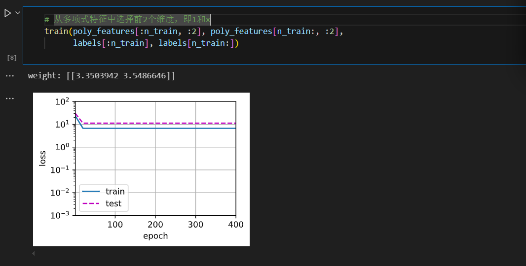
展示欠拟合(线性函数拟合)
再看看线性函数拟合,减少该模型的训练损失相对困难。在最后一个迭代周期完成后,训练损失仍然很高。当用来拟合非线性模式(如这里的三阶多项式函数)时,线性模型容易欠拟合。
# 从多项式特征中选择前2个维度,即1和x
train(poly_features[:n_train, :2], poly_features[n_train:, :2],
      labels[:n_train], labels[n_train:])
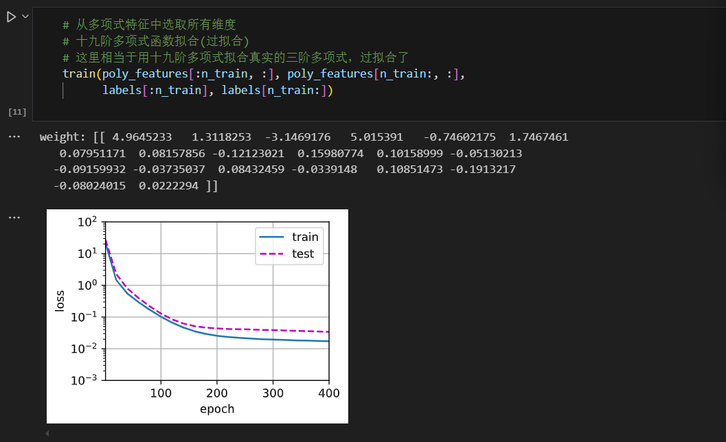
展示过拟合(高阶多项式函数拟合)
尝试使用一个阶数过高的多项式来训练模型。在这种情况下,没有足够的数据用于学到高阶系数应该具有接近于零的值。因此,这个过于复杂的模型会轻易受到训练数据中噪声的影响。虽然训练损失可以有效地降低,但测试损失仍然很高。结果表明,复杂模型对数据造成了过拟合。
# 从多项式特征中选取所有维度
# 十九阶多项式函数拟合(过拟合)
# 这里相当于用十九阶多项式拟合真实的三阶多项式,过拟合了
train(poly_features[:n_train, :], poly_features[n_train:, :],
      labels[:n_train], labels[n_train:])
QA 思考
Q1: SVM 的缺点是啥?
A1:SVM 是通过 Kernel 来匹配模型复杂度的,使用 Kernel SVM 算起来不容易,也就是 SVM 很难做到100万个数据点,但是对于多层感知机的话通过梯度下降是很容易做到这么多的数据点的。 SVM 可调节的东西不多,可调性不行。
Q2:k折交叉验证的目的是确定超参数吗?然后还要用这个超参数再训练一遍全数数据吗?
A2:有以下几种做法:
- 第一种做法:k 折交叉验证就是来确定一个超参数,确定好之后我在整个数据集上再全部训练一次
- 第二种做法:不再重新训练了,直接找选定超参数后K折里精度最好(或随便)的一折,选择该模型,不再重新训练。代价就是少看了一些训练集,模型的训练就是稍微少了一点点。
- 第三种做法:把 k 折交叉验证的 k 个模型全部拿下来,真的做预测的时候,把一个测试数据集全部全部放到 k 个模型中,每一个都预测一次
后记
根据上述的理解,写了一段不依赖于 d2l 的代码,同时可以在Pycharm上面运行。
import math
import numpy as np
import torch
from matplotlib import pyplot as plt
from torch import nn
from torch.utils.data import DataLoader, TensorDataset


class Animator:
    def __init__(self, xlabel=None, ylabel=None, legend=None, xlim=None,
                 ylim=None, xscale='linear', yscale='linear',
                 fmts=('-', 'm--', 'g-.', 'r:'), figsize=(3.5, 2.5)):
        if legend is None:
            legend = []
        self.xlabel = xlabel
        self.ylabel = ylabel
        self.legend = legend
        self.xlim = xlim
        self.ylim = ylim
        self.xscale = xscale
        self.yscale = yscale
        self.fmts = fmts
        self.figsize = figsize
        self.X, self.Y = [], []

    def add(self, x, y):
        if not hasattr(y, "__len__"):
            y = [y]
        n = len(y)
        if not hasattr(x, "__len__"):
            x = [x] * n
        if not self.X:
            self.X = [[] for _ in range(n)]
        if not self.Y:
            self.Y = [[] for _ in range(n)]
        for i, (a, b) in enumerate(zip(x, y)):
            if a is not None and b is not None:
                self.X[i].append(a)
                self.Y[i].append(b)

    def show(self):
        plt.figure(figsize=self.figsize)
        for x_data, y_data, fmt in zip(self.X, self.Y, self.fmts):
            plt.plot(x_data, y_data, fmt)
        plt.xlabel(self.xlabel)
        plt.ylabel(self.ylabel)
        if self.legend:
            plt.legend(self.legend)
        if self.xlim:
            plt.xlim(self.xlim)
        if self.ylim:
            plt.ylim(self.ylim)
        plt.xscale(self.xscale)
        plt.yscale(self.yscale)
        plt.grid()
        plt.show()


class Accumulator:
    # 若需要同时累积两个指标 ,则可以初始化为 Accumulator(2) 会创建一个列表 [0.0,0.0]
    def __init__(self, n):
        self.data = [0.0] * n

    # 假设当前 self.data = [1.0, 2.0],调用 add(3.0, 4.0) 后,self.data 会变为 [4.0, 6.0]
    def add(self, *args):
        self.data = [a + float(b) for a, b in zip(self.data, args)]

    def reset(self):
        self.data = [0.0] * len(self.data)

    # 返回 self.data 中对应位置的元素
    def __getitem__(self, idx):
        return self.data[idx]


def evaluate_loss(net, data_iter, loss):
    metric = Accumulator(2)
    for X, y in data_iter:
        out = net(X)
        y = y.reshape(out.shape)
        l = loss(out, y)
        metric.add(l.sum(), l.numel())
    return metric[0] / metric[1]


# 预测正确的数量
def accuracy(y_hat, y):
    if len(y_hat.shape) > 1 and y_hat.shape[1] > 1:
        y_hat = y_hat.argmax(axis=1)
    cmp = y_hat.type(y.dtype) == y
    return float(cmp.type(y.dtype).sum())


def train_epoch_ch3(net, train_iter, loss, updater):
    if isinstance(net, torch.nn.Module):
        net.train()
    metric = Accumulator(3)
    for X, y in train_iter:
        y_hat = net(X)
        l = loss(y_hat, y)
        if isinstance(updater, torch.optim.Optimizer):
            updater.zero_grad()
            l.mean().backward()
            updater.step()
        else:
            l.sum().backward()
            updater(X.shape[0])
        metric.add(float(l.sum()), accuracy(y_hat, y), y.numel())
    return metric[0] / metric[2], metric[1] / metric[2]


def train(train_features, test_features, train_labels, test_labels,
          num_epochs=400):
    # 定义损失函数(均方误差)
    loss = nn.MSELoss(reduction='mean')  # 使用 'mean' 计算平均损失
    # 获取输入特征的维度
    input_shape = train_features.shape[-1]
    # 无需偏置
    net = nn.Sequential(nn.Linear(input_shape, 1, bias=False))
    # 设置批量大小
    batch_size = min(10, train_labels.shape[0])
    # 将数据集转化为 DataLoader
    train_dataset = TensorDataset(train_features, train_labels.reshape(-1, 1))
    train_iter = DataLoader(train_dataset, batch_size=batch_size, shuffle=True)

    test_dataset = TensorDataset(test_features, test_labels.reshape(-1, 1))
    test_iter = DataLoader(test_dataset, batch_size=batch_size, shuffle=False)
    # 定义优化器(SGD)
    trainer = torch.optim.SGD(net.parameters(), lr=0.01)

    animator = Animator(xlabel='epoch', ylabel=loss, yscale='log',
                        xlim=[1, num_epochs], ylim=[1e-3, 1e2],
                        legend=['train', 'loss'])

    for epoch in range(num_epochs):
        train_epoch_ch3(net, train_iter, loss, trainer)
        if epoch == 0 or (epoch + 1) % 20 == 0:
            animator.add(epoch + 1, (evaluate_loss(net, train_iter, loss),
                                     evaluate_loss(net, test_iter, loss)))
    animator.show()
    # 打印最终学习到的权重
    print('weight:', net[0].weight.data.numpy())


if __name__ == "__main__":
    max_degree = 20
    n_train, n_test = 100, 100
    true_w = np.zeros(max_degree)
    true_w[0:4] = np.array([5, 1.2, -3.4, 5.6])

    features = np.random.normal(size=(n_train + n_test, 1))
    np.random.shuffle(features)  # 打乱顺序

    poly_features = np.power(features, np.arange(max_degree).reshape(1, -1))

    for i in range(max_degree):
        poly_features[:, i] /= math.gamma(i + 1)

        labels = np.dot(poly_features, true_w)
        labels += np.random.normal(scale=0.1, size=labels.shape)

    true_w, features, poly_features, labels = [torch.tensor(x, dtype=torch.float32)
                                               for x in [true_w, features, poly_features, labels]]

    print("features = {}, poly_features = {}, labels = {}".format(features[:2], poly_features[:2, :], labels[:2]))

    # 从多项式特征中选择前4个维度,即1,x,x^2/2!,x^3/3!
    train(poly_features[:n_train, :4], poly_features[n_train:, :4],
          labels[:n_train], labels[n_train:])

    # 从多项式特征中选择前2个维度,即1和x
    train(poly_features[:n_train, :2], poly_features[n_train:, :2],
          labels[:n_train], labels[n_train:])

    # 从多项式特征中选取所有维度
    # 十九阶多项式函数拟合(过拟合)
    # 这里相当于用十九阶多项式拟合真实的三阶多项式,过拟合了
    train(poly_features[:n_train, :], poly_features[n_train:, :],
          labels[:n_train], labels[n_train:])


 553
553

 被折叠的 条评论
为什么被折叠?
被折叠的 条评论
为什么被折叠?
 到【灌水乐园】发言


