


#PINN#、#PDE#、#深度学习#
文章目录
简介
本人是做化工模拟的一名学生,最近在学习PINN(Physics-Informed Neural Networks,物理信息神经网络)对管道动力学进行建模研究,PINN由于其对机理与数据的良好兼顾性非常热门,本文是作者对PINN入门研究过程的一个练手小题目,main code也是作者代码是基于pytorch2.6.0写的,发上来供各位参考,欢迎研究管道动力学和PINN的小伙伴一起讨论~
一、PINN简介
1.1PINN原理
PINN是一种结合了深度学习和物理学知识的机器学习模型,它通过将物理定律(通常以偏微分方程的形式)嵌入到神经网络的训练过程中,实现对物理现象的精确模拟和预测。这种模型不仅能够从数据中学习,还能确保预测结果符合物理规律,从而在数据稀缺或噪声较大的情况下,仍然能够进行有效的训练和预测。
1.2PINN步骤
-
定义物理问题和相应的物理定律:首先,需要明确所要解决的问题及其背后的物理原理,例如热传导、流体力学等,并将其转化为一组偏微分方程。
-
构建神经网络架构:根据问题的复杂程度,设计合适的神经网络结构,作为函数的逼近器。神经网络的输入通常是空间坐标、时间等变量,输出则是预测的物理量。
-
编码边界条件:将初始条件、边界值等物理约束编码到神经网络的损失函数中。这通常通过在网络的输入和输出上设置特定点的期望值来实现。
-
定义损失函数:损失函数是PINN模型训练中的关键部分,它包含数据误差项和物理信息误差项。数据误差项用于衡量网络预测值与真实数据之间的差异,而物理信息误差项则用于衡量网络预测值是否满足物理定律。通过调整这两项在损失函数中的权重,可以平衡数据拟合和物理约束的重要性。
-
训练网络:采用梯度下降或其他优化算法,最小化损失函数,同时更新神经网络的权重。在训练过程中,物理定律作为先验知识,为神经网络提供了额外的指导信息,使其能够更有效地学习和泛化。
-
验证结果:检查训练得到的网络解是否满足物理定律和边界条件,并通过可视化和数值测试评估其精度。
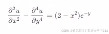
二、问题描述
2.1求解的偏微分方程
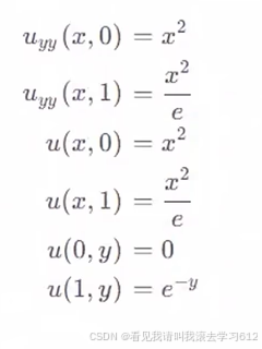
2.2偏微分方程的边界条件
三、基于pytorch2.6.0框架的代码实现
3.1初始条件设定
"""西南石油大学  major:chemical engineering   @author:zhujy
简单的一个PINN求解偏微分方程实例"""

import torch
import matplotlib.pyplot as plt


epochs = 10000 # 训练代数

# 画图所需参数
h = 100  # 画图网格密度
N = 1000  # 内点的点数
N1 = 100  # 边界点的点数
N2 = 1000  # PDE的数据点


# 设置初始seed值,确保每次运行结果一样
def setup_seed(seed):
    torch.manual_seed(seed)


# 我的电脑没显卡,只能这样设置了。。。

# 设置随机数种子,设定固定的随机数以便结果可以复现
setup_seed(888888)
3.2边界条件设定
# 规定边界条件以及对内点采样
def interior(n=N):
    # 内点
    x = torch.rand(n, 1)
    y = torch.rand(n, 1)
    cond = (2 - x ** 2) * torch.exp(-y)
    return x.requires_grad_(True), y.requires_grad_(True), cond


# 希望追踪x,y的参数,并计算它们的梯度

def down_yy(n=N1):
    # 边界条件1
    x = torch.rand(n, 1)
    y = torch.zeros_like(x)  # zeros_like和one_like 都是用全矩阵为0和1
    cond = x ** 2
    return x.requires_grad_(True), y.requires_grad_(True), cond


def up_yy(n=N1):
    # 边界条件2
    x = torch.rand(n, 1)
    y = torch.ones_like(x)
    cond = x ** 2 / torch.e
    return x.requires_grad_(True), y.requires_grad_(True), cond


def down(n=N1):
    # 边界条件3、
    x = torch.rand(n, 1)
    y = torch.zeros_like(x)
    cond = x ** 2
    return x.requires_grad_(True), y.requires_grad_(True), cond


def up(n=N1):
    # 边界条件4
    x = torch.rand(n, 1)
    y = torch.ones_like(x)
    cond = x ** 2 / torch.e
    return x.requires_grad_(True), y.requires_grad_(True), cond


def left(n=N1):
    # 边界条件5
    y = torch.rand(n, 1)
    x = torch.zeros_like(y)
    cond = torch.zeros_like(x)
    return x.requires_grad_(True), y.requires_grad_(True), cond


def right(n=N1):
    # 边界条件6
    y = torch.rand(n, 1)
    x = torch.ones_like(y)
    cond = torch.exp(-y)
    return x.requires_grad_(True), y.requires_grad_(True), cond


# 对内点进行处理
def data_interior(n=N2):
    x = torch.rand(n, 1)
    y = torch.rand(n, 1)
    cond = (x ** 2) * torch.exp(-y)
    return x.requires_grad_(True), y.requires_grad_(True), cond
3.3搭建PINN神经网络
# 搭建Neural Network
# 神经网络是2个输入,到一个输出,中间有三个隐藏层,每层32个神经元
# MLP是最基础的全连接神经网络(多层感知机)
# 激活函数选择Tanh
class MLP(torch.nn.Module):
    def __init__(self):
        super(MLP, self).__init__()
        self.net = torch.nn.Sequential(
            torch.nn.Linear(2, 32),
            torch.nn.Tanh(),
            torch.nn.Linear(32, 32),
            torch.nn.Tanh(),
            torch.nn.Linear(32, 32),
            torch.nn.Tanh(),
            torch.nn.Linear(32, 32),
            torch.nn.Tanh(),
            torch.nn.Linear(32, 1),
        )

    def forward(self, x):
        return self.net(x)
3.4构造损失函数
# 规定损失函数LOSS,LOSS由两部分构成,一部分是数据误差,一部分是方程误差
# 损失函数使用MSE均方方差,每个数据点所产生的方差的平均值

loss = torch.nn.MSELoss()


# 规定梯度,order为阶数,高阶偏导利用嵌套求解
def gradients(u, x, order=1):
    if order == 1:
        return torch.autograd.grad(u, x, grad_outputs=torch.ones_like(u), create_graph=True, only_inputs=True, )[0]
    else:
        return gradients(gradients(u, x), x, order=order - 1)


# 计算PDE的损失
def l_interior(u):
    # 内点的损失函数
    # uxy就是u(x,y)是预测值,cond是真实值
    x, y, cond = interior()
    uxy = u(torch.cat([x, y], dim=1))
    # torch.cat函数是将两个元素按一定规律拼接起来
    return loss(gradients(uxy, x, 2) - gradients(uxy, y, 4), cond)


def l_down_yy(u):
    # 边界条件1的损失函数
    x, y, cond = down_yy()
    uxy = u(torch.cat([x, y], dim=1))
    # torch.cat函数是将两个元素按一定规律拼接起来
    return loss(gradients(uxy, y, 2), cond)


def l_up_yy(u):
    # 边界条件2的损失函数
    x, y, cond = up_yy()
    uxy = u(torch.cat([x, y], dim=1))
    # torch.cat函数是将两个元素按一定规律拼接起来
    return loss(gradients(uxy, y, 2), cond)


def l_down(u):
    # 边界条件3的损失函数
    x, y, cond = down()
    uxy = u(torch.cat([x, y], dim=1))
    # torch.cat函数是将两个元素按一定规律拼接起来
    return loss(uxy, cond)


def l_up(u):
    # 边界条件4的损失函数
    x, y, cond = up()
    uxy = u(torch.cat([x, y], dim=1))
    # torch.cat函数是将两个元素按一定规律拼接起来
    return loss(uxy, cond)


def l_left(u):
    # 边界条件5的损失函数
    x, y, cond = left()
    uxy = u(torch.cat([x, y], dim=1))
    # torch.cat函数是将两个元素按一定规律拼接起来
    return loss(uxy, cond)


def l_right(u):
    # 边界条6的损失函数
    x, y, cond = right()
    uxy = u(torch.cat([x, y], dim=1))
    # torch.cat函数是将两个元素按一定规律拼接起来
    return loss(uxy, cond)


# 构造数据损失
def l_data(u):
    x, y, cond = data_interior()
    uxy = u(torch.cat([x, y], dim=1))
    return loss(uxy, cond)
3.5进行Training
# 训练Training
u = MLP()
opt = torch.optim.Adam(params=u.parameters(),lr=0.001)
# 初始化模型参数,并将它们传入Adam函数,构造出一个Adam优化器
# 可以通过给定lr的数值来确定学习率
loss_history = []

for i in range(epochs):
    opt.zero_grad()
    # 将这一轮的梯度清零,防止影响下一轮的更新
    LOSS = l_interior(u) + l_up_yy(u) + l_down_yy(u) + l_up(u) + l_down(u) + l_left(u) + l_right(u) + l_data(u)
    LOSS.backward()
    # 反向计算出各参数的梯度
    opt.step()
    # 更新网络中的参数
    loss_history.append(LOSS.item())
    # 记录当前epoch的损失值
    if i % 10 == 0:
        print(i,'LOSS:',LOSS.item())
# 绘制损失曲线
plt.plot(loss_history)
plt.xlabel('Epoch')
plt.ylabel('Loss')
plt.title('Training Loss Curve')
plt.grid(True)  # 可选,添加网格线以便更好地观察趋势
plt.show()
3.6预测与验证
# predict
xc = torch.linspace(0, 1, h)
xm, ym = torch.meshgrid(xc, xc)
xx = xm.reshape(-1, 1)
yy = ym.reshape(-1, 1)
xy = torch.cat([xx, yy], dim=1)
u_pred = u(xy)
u_real = xx * xx * torch.exp(-yy)
u_error = torch.abs(u_pred - u_real)
u_pred_fig = u_pred.reshape(h, h)
u_real_fig = u_real.reshape(h, h)
u_error_fig = u_error.reshape(h, h)
print("最大误差为:", float(torch.max(u_error)))
print(xx)
print(xy)
3.7结果可视化
绘制损失函数收敛曲线等结果图
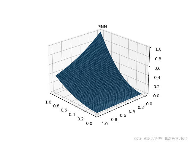
# 作图
# 图一PINN数值解图
fig = plt.figure(1)
ax = fig.add_subplot(111, projection='3d')
ax.plot_surface(xm.detach().numpy(), ym.detach().numpy(), u_pred_fig.detach().numpy())
ax.text2D(0.5, 0.9, 'PINN', transform=ax.transAxes)
plt.show()
fig.savefig("PINN solve.png")
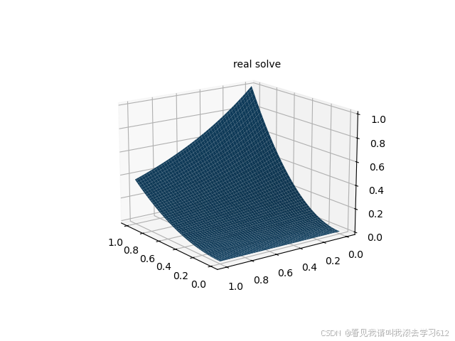
# 做真实解图
fig = plt.figure(2)
ax = fig.add_subplot(111, projection='3d')
ax.plot_surface(xm.detach().numpy(), ym.detach().numpy(), u_real_fig.detach().numpy())
ax.text2D(0.5, 0.9, 'real solve', transform=ax.transAxes)
plt.show()
fig.savefig("real solve.png")
# 误差图
fig = plt.figure(3)
ax = fig.add_subplot(111, projection='3d')
ax.plot_surface(xm.detach().numpy(), ym.detach().numpy(), u_error_fig.detach().numpy())
ax.text2D(0.5, 0.9, 'abs error', transform=ax.transAxes)
plt.show()
fig.savefig("abs error.png")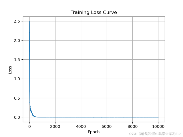


 8956
8956

 被折叠的 条评论
为什么被折叠?
被折叠的 条评论
为什么被折叠?
 到【灌水乐园】发言


