


 探讨了阿里天池举办的工业蒸汽量预测竞赛,内容覆盖数据探索、特征工程、多种模型应用及模型融合策略。通过分钟级锅炉传感器数据,运用机器学习算法如梯度提升树、LightGBM、Xgboost、随机森林和SVR等,优化预测模型,最终实现蒸汽量高效预测,强调模型融合提升预测精度。
AI竞赛3-阿里天池工业蒸汽量预测
1.天池工业蒸汽量-数据探索
1.1 项目介绍
- 火力发电的基本原理是:燃料在燃烧时加热水生成蒸汽,蒸汽压力推动汽轮机旋转,然后汽轮机带动发电机旋转产生电能。在这一系列的能量转化中,影响发电效率的核心是锅炉的燃烧效率,即燃料燃烧加热水产生高温高压蒸汽。锅炉的燃烧效率的影响因素很多,包括锅炉的可调参数,如燃烧给量、一二次风、引风、返料风、给水水量;以及锅炉的工况,比如锅炉床温、床压、炉膛温度、压力、过热器温度等。经脱敏后的锅炉传感器采集的数据(采集频率是分钟级别),根据锅炉的工况,预测产生的蒸汽量。

1.2 数据探索工具包
import numpy as np
import pandas as pd
import matplotlib.pyplot as plt
import seaborn as sns
from scipy import stats
import warnings
warnings.filterwarnings("ignore")
1.3 数据加载
train_data_file = "./zhengqi_train.txt"
test_data_file =  "./zhengqi_test.txt"
train_data = pd.read_csv(train_data_file, sep='\t')
test_data = pd.read_csv(test_data_file, sep='\t')
1.4 数据查看
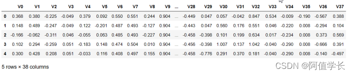
test_data.head()
train_data.info()
<class 'pandas.core.frame.DataFrame'>
RangeIndex: 2888 entries, 0 to 2887
Data columns (total 39 columns):
 #   Column  Non-Null Count  Dtype
---  ------  --------------  -----
 0   V0      2888 non-null   float64
 1   V1      2888 non-null   float64
 2   V2      2888 non-null   float64
...
 36  V36     2888 non-null   float64
 37  V37     2888 non-null   float64
 38  target  2888 non-null   float64
dtypes: float64(39)
memory usage: 880.1 KB

test_data.info()
<class 'pandas.core.frame.DataFrame'>
RangeIndex: 1925 entries, 0 to 1924
Data columns (total 38 columns):
 #   Column  Non-Null Count  Dtype
---  ------  --------------  -----
 0   V0      1925 non-null   float64
 1   V1      1925 non-null   float64
 2   V2      1925 non-null   float64
...
 36  V36     1925 non-null   float64
 37  V37     1925 non-null   float64
dtypes: float64(38)
memory usage: 571.6 KB

# 此训练集数据共有2888个样本,测试集数据共有1925个样本,数据中有V0-V37共计38个特征变量,变量类型都为数值类型,所有数据特征没有缺失值数据; 数据字段由于采用脱敏处理,删除特征数据具体含义;target字段为标签变量
1.5 数据统计信息查看
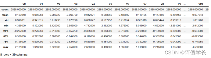
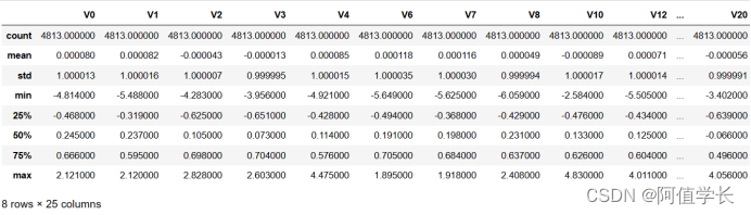
train_data.describe()
# 下面数据显示数据的统计信息,例如样本数、数据均值mean、标准差std、最小值、最大值等
1.6 数据字段信息查看
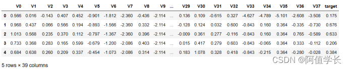
train_data.head()
# 下面显示训练集前5条数据基本信息,数据都是浮点型数据,数据都是数值型连续型特征
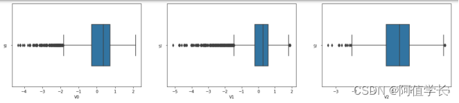
1.7 数据探索-箱式图
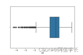
(1) 第一个特征箱式图
fig = plt.figure(figsize=(6, 4))  # 指定绘图对象宽度和高度
sns.boxplot(train_data['V0'],width=0.5)
plt.savefig('./2-特征箱式图.jpg',dpi = 200)
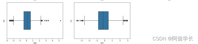
(2) 全部特征箱式图
column = train_data.columns.tolist()[:39]  # 列表头
fig = plt.figure(figsize=(20, 60))   # 指定绘图对象宽度和高度
for i in range(38):
    plt.subplot(13, 3, i + 1)   # 13行3列子图
    sns.boxplot(train_data[column[i]], width=0.5)   # 箱式图
    plt.ylabel(column[i], fontsize=8)
1.8 数据分布查看
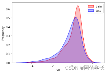
1.8.1 对比同一特征变量‘V0’下训练集数据和测试集数据分布情况
ax = sns.kdeplot(train_data['V0'], color="Red", shade=True)
ax = sns.kdeplot(test_data['V0'], color="Blue", shade=True)
ax.set_xlabel('V0')
ax.set_ylabel("Frequency")
ax = ax.legend(["train","test"])
plt.savefig('./3-数据分布.jpg',dpi = 200)
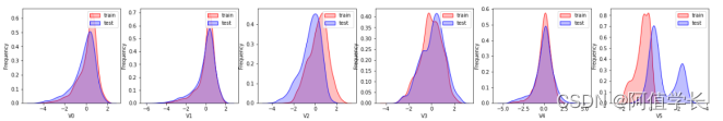
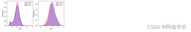
1.8.2 所有特征变量下训练集数据和测试集数据数据分布情况
dist_cols = 6
dist_rows = len(test_data.columns)//6 + 1
plt.figure(figsize=(4*dist_cols,4*dist_rows))
i=1
for col in test_data.columns:
    ax=plt.subplot(dist_rows,dist_cols,i)
    ax = sns.kdeplot(train_data[col], color="Red", shade=True)
    ax = sns.kdeplot(test_data[col], color="Blue", shade=True)
    ax.set_xlabel(col)
    ax.set_ylabel("Frequency")
    ax = ax.legend(["train","test"])
    i+=1
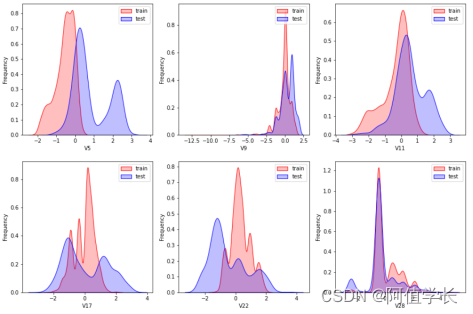
1.8.3 查看特征'V5', 'V17', 'V28', 'V22', 'V11', 'V9'数据分布
col = 3
row = 2
plt.figure(figsize=(5 * col,5 * row))
i=1
for c in ["V5","V9","V11","V17","V22","V28"]:
    ax = plt.subplot(row,col,i)
    ax = sns.kdeplot(train_data[c], color="Red", shade=True)
    ax = sns.kdeplot(test_data[c], color="Blue", shade=True)
    ax.set_xlabel(c)
    ax.set_ylabel("Frequency")
    ax = ax.legend(["train","test"])
    i+=1
plt.savefig('./4-数据分布.jpg',dpi = 200)

# 由下图数据分布可看到特征'V5','V9','V11','V17','V22','V28' 训练集数据与测试集数据分布不一致,会导致模型泛化能力差,故删除此类特征
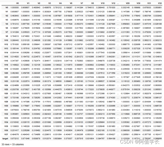
1.9 特征相关性
1.9.1 特征、标签相关性
drop_col_kde = ['V5','V9','V11','V17','V22','V28']
train_data_drop = train_data.drop(drop_col_kde, axis=1)
train_corr = train_data_drop.corr()
train_corr
1.9.2 热力图绘制
ax = plt.subplots(figsize=(20, 16))  # 调整画布大小
ax = sns.heatmap(train_corr, vmax=.8, square=True, annot=True) # 画热力图   annot=True 显示系数
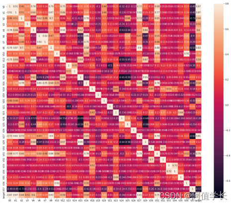
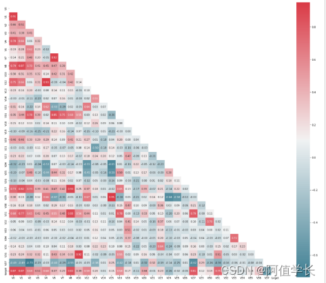
1.9.3 半热力图
plt.figure(figsize=(24, 20))  # 指定绘图对象宽度和高度
colnm = train_data_drop.columns.tolist()  # 列表头
mcorr = train_data_drop.corr()    # 相关系数矩阵,即给出任意两个变量之间的相关系数
mask = np.zeros_like(mcorr, dtype=np.bool) # False  # 构造与mcorr同维数矩阵为bool类型
mask[np.triu_indices_from(mask)] = True  # 角分线右侧为True,右上角设置为True  (戴面具,看不见)
cmap = sns.diverging_palette(220, 10, as_cmap=True)  # 设置colormap对象,表示颜色
g = sns.heatmap(mcorr, mask=mask, cmap=cmap, square=True, annot=True, fmt='0.2f')  # 热力图(看两两相似度)
plt.savefig('./5-特征相关性.jpg',dpi = 400)

# 下图为所有特征变量和target变量两两之间的相关系数,由此可看出各个特征变量V0-V37之间的相关性以及特征变量V0-V37与target的相关性
np.triu_indices_from(mask)
(array([ 0,  0,  0,  0,  0,  0,  0,  0,  0,  0,  0,  0,  0,  0,  0,  0,  0,
         0,  0,  0,  0,  0,  0,  0,  0,  0,  0,  0,  0,  0,  0,  0,  0,  1,
...
        25, 25, 25, 25, 25, 25, 26, 26, 26, 26, 26, 26, 26, 27, 27, 27, 27,
        27, 27, 28, 28, 28, 28, 28, 29, 29, 29, 29, 30, 30, 30, 31, 31, 32]),
 array([ 0,  1,  2,  3,  4,  5,  6,  7,  8,  9, 10, 11, 12, 13, 14, 15, 16,
        17, 18, 19, 20, 21, 22, 23, 24, 25, 26, 27, 28, 29, 30, 31, 32,  1,
...
        27, 28, 29, 30, 31, 32, 26, 27, 28, 29, 30, 31, 32, 27, 28, 29, 30,
        31, 32, 28, 29, 30, 31, 32, 29, 30, 31, 32, 30, 31, 32, 31, 32, 32]))

mask
array([[ True,  True,  True, ...,  True,  True,  True],
       [False,  True,  True, ...,  True,  True,  True],
       [False, False,  True, ...,  True,  True,  True],
       ...,
       [False, False, False, ...,  True,  True,  True],
       [False, False, False, ..., False,  True,  True],
       [False, False, False, ..., False, False,  True]])
1.10 特征筛选
1.10.1 特征删除-数据分布
train_data.drop(drop_col_kde,axis = 1,inplace=True) # 删除训练数据和预测数据
test_data.drop(drop_col_kde,axis = 1,inplace= True)
train_data.head()

1.10.2 特征筛选-相关性系数
相关性系数:
(1) 0.8-1.0 极强相关;
(2) 0.6-0.8 强相关;
(3) 0.4 -0.6 中等程度相关;
(4) 0.2-0.4 弱相关;
(5) 0.0-0.2 极弱相关或无相关(过滤极弱相关的特征)
过滤条件特征相关性系数:小于0.1
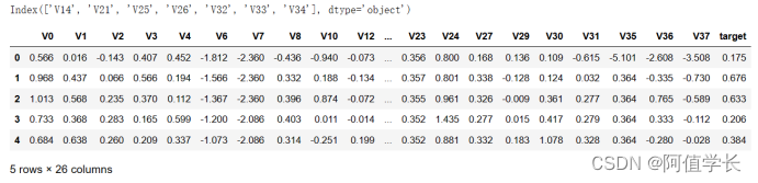
cond = mcorr['target'].abs() < 0.1
drop_col_corr = mcorr.index[cond]
display(drop_col_corr)
train_data.drop(drop_col_corr,axis = 1,inplace=True) # 删除
test_data.drop(drop_col_corr,axis = 1,inplace=True)
display(train_data.head())
1.10.3 训练、测试数据合并保存
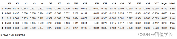
train_data['label'] = 'train'
test_data['label'] = 'test'
all_data = pd.concat([train_data,test_data])
all_data.to_csv('./processed_zhengqi_data.csv',index=False)
all_data.head()
2.天池工业蒸汽量-特征工程
2.1 数据分析工具包
import numpy as np
import pandas as pd
import matplotlib.pyplot as plt
import seaborn as sns
from scipy import stats
from sklearn import preprocessing
import warnings
warnings.filterwarnings("ignore")
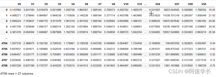
2.2 数据加载
all_data = pd.read_csv('./processed_zhengqi_data.csv')
display(all_data.head())
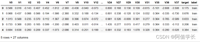
all_data.shape
(4813, 27)
2.3 最大小值归一化
2.3.1 归一化之前
columns=list(all_data.columns) # 特征归一化
columns.remove('label') # 删除标签列索引
columns.remove('target') # 删除目标值
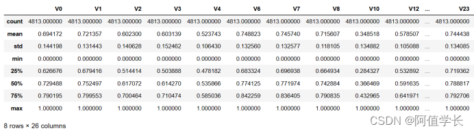
all_data[columns].describe()
2.3.2 最大小值归一化
def norm_min_max(col):  # 定义归一化方法
    return (col-col.min())/(col.max()-col.min())
all_data[columns] = all_data[columns].apply(norm_min_max,axis=0)
all_data.describe()
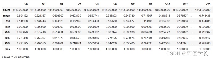
2.3.3 最大小值归一化-sklearn
from sklearn import preprocessing
min_max_scaler = preprocessing.MinMaxScaler()
all_data[columns] = min_max_scaler.fit_transform(all_data[columns]) # 处理完后数据变换为Numpy数组
all_data[columns] = pd.DataFrame(all_data,columns=columns)
all_data.describe()
2.4 数据正态化(Box-Cox变换)
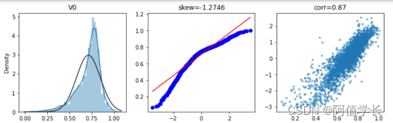
# 查看特征变量‘V0’的数据分布直方图、并绘制Q-Q图查看数据是否近似于正态分布、特征目标值相关性
2.4.1 训练数据获取
cond = all_data['label'] == 'train'
train_data = all_data[cond]
train_data.drop(labels='label',axis = 1,inplace=True)
2.4.2 'V0'三图可视化
plt.figure(figsize=(12,4))
ax = plt.subplot(1,3,1)  # 绘制直方图
sns.distplot(train_data['V0'],fit=stats.norm)  # 拟合标准正态分布
ax = plt.subplot(1,3,2)  # 绘制Q-Q图
stats.probplot(train_data['V0'],plot = ax)  # 生成样本数据相对于指定理论分布(默认正态分布)的分位数的概率图
plt.title('skew='+'{:.4f}'.format(stats.skew(train_data['V0'])))
ax = plt.subplot(1,3,3)  # 绘制特征和目标值相关性散点图
plt.scatter(train_data['V0'], train_data['target'],s = 5,alpha=0.5)
plt.title('corr='+'{:.2f}'.format(np.corrcoef(train_data['V0'],train_data['target'])[0][1]))
plt.savefig('./6-Box-Cox.jpg',dpi = 200)
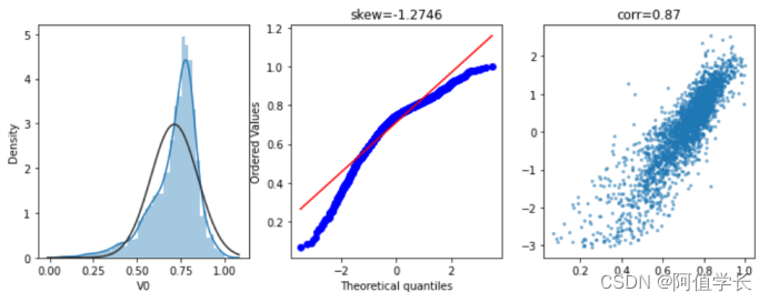
#    skew函数计算数据集的偏度:
(1) skew = 0,正态分布
(2) skew > 0,向右偏移
(3) skew < 0,向左偏移
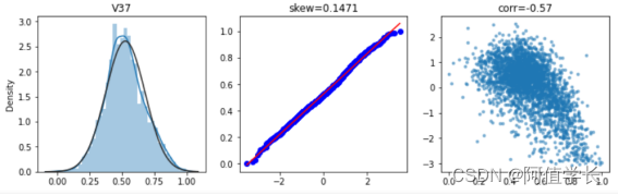
2.4.3 所有特征三图可视化
fcols = 3
columns = list(train_data.columns)
columns.remove('target')
frows = len(columns)
plt.figure(figsize=(4*fcols,4*frows))
i=0
for col in columns:
    feature = train_data[[col, 'target']]
    i+=1
    plt.subplot(frows,fcols,i)
    sns.distplot(feature[col] , fit=stats.norm);
    plt.title(col)
    plt.xlabel('')
    i+=1
    plt.subplot(frows,fcols,i)
    _=stats.probplot(feature[col], plot=plt)
    plt.title('skew='+'{:.4f}'.format(stats.skew(feature[col])))
    plt.xlabel('')
    plt.ylabel('')
    i+=1
    plt.subplot(frows,fcols,i)
    plt.plot(feature[col], feature['target'],'.',alpha=0.5)
    plt.title('corr='+'{:.2f}'.format(np.corrcoef(feature[col], feature['target'])[0][1]))
2.4.4 特征Box-Cox变换
fcols = 6 # 绘图显示Box-Cox变换对数据分布影响
columns = list(train_data.columns)  # Box-Cox变换:改善数据正态性、对称性和方差相等性
columns.remove('target')
frows = len(columns)
plt.figure(figsize=(4*fcols,4*frows))
i=0
def norm_min_max(feature):
    return (feature-feature.min())/(feature.max()-feature.min())
for col in columns:
    feature = train_data[[col, 'target']].dropna()
    i+=1
    plt.subplot(frows,fcols,i)
    sns.distplot(feature[col] , fit=stats.norm);
    plt.title(col+' raw')
    plt.xlabel('')
    i+=1
    plt.subplot(frows,fcols,i)
    _=stats.probplot(feature[col], plot=plt)
    plt.title('skew='+'{:.4f}'.format(stats.skew(feature[col])))
    plt.xlabel('')
    plt.ylabel('')
    i+=1
    plt.subplot(frows,fcols,i)
    plt.plot(feature[col], feature['target'],'.',alpha=0.5)
    plt.title('corr='+'{:.2f}'.format(np.corrcoef(feature[col], feature['target'])[0][1]))
    i+=1
    plt.subplot(frows,fcols,i)
    trans_feature, lambda_feature = stats.boxcox(feature[col].dropna()+1) # Box-Cox变换
    trans_feature = norm_min_max(trans_feature)
    sns.distplot(trans_feature , fit=stats.norm);
    plt.title(col+' Tramsformed')
    plt.xlabel('')
    i+=1
    plt.subplot(frows,fcols,i)
    _=stats.probplot(trans_feature, plot=plt)
    plt.title('skew='+'{:.4f}'.format(stats.skew(trans_feature)))
    plt.xlabel('')
    plt.ylabel('')
    i+=1
    plt.subplot(frows,fcols,i)
    plt.plot(trans_feature, feature['target'],'.',alpha=0.5)
    plt.title('corr='+'{:.2f}'.format(np.corrcoef(trans_feature,feature['target'])[0][1]))
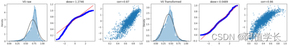
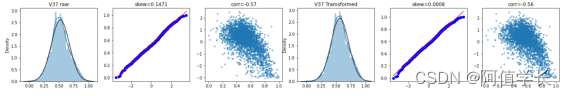
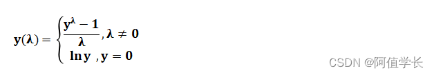
# 从回归结果可见经过Box-Cox变换数据分布更加正态化,所以进行Box-Cox变换很有必要。Box-Cox变换是Box和Cox在1964年提出的一种广义幂变换方法,是统计建模中常用的一种数据变换:用于连续的响应变量不满足正态分布的情况,Box-Cox变换一般形式:
columns=list(all_data.columns)
columns.remove('label') # 删除标签列索引
columns.remove('target') # 删除目标值
for col in columns:
    all_data.loc[:,col], _ = stats.boxcox(all_data.loc[:,col]+1) # 进行Box-Cox变换
2.5 数据获取
from sklearn.model_selection import train_test_split
def get_train_data():
    train_data = all_data[all_data["label"]=="train"]
    y = train_data.target  # 数据拆分:训练数据和验证数据
    X = train_data.drop(["label","target"],axis=1)
    return X,y
#(1) 提取训练和验证数据
def split_train_data():
    train_data = all_data[all_data["label"]=="train"]
    y = train_data.target
    X = train_data.drop(["label","target"],axis=1)
    X_train,X_valid,y_train,y_valid=train_test_split(X,y,test_size=0.2)
    return X_train,X_valid,y_train,y_valid
#(2) 提取预测数据
def get_test_data():
    test_data = all_data[all_data["label"]=="test"].reset_index(drop=True)
    return test_data.drop(["label","target"],axis=1)
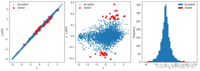
2.6 异常值过滤
from sklearn.metrics import mean_squared_error # 基于模型预测的异常值检测
def find_outliers(model, X, y, sigma = 3):
model.fit(X,y) # 模型训练
y_pred = pd.Series(model.predict(X), index=y.index)
resid = y - y_pred # 计算预测值和真实值之差
mean_resid = resid.mean()
std_resid = resid.std()
z = (resid - mean_resid)/std_resid # 异常值计算 Z-score归一化
outliers = z[abs(z)>sigma].index # 正太分布异常值过滤:3σ法则
print('R2=',model.score(X,y)) # 输出模型评价
print("mse=",mean_squared_error(y,y_pred))
print('---------------------------------------')
print('mean of residuals:',mean_resid) # 残差数据
print('std of residuals:',std_resid)
print('---------------------------------------')
print(len(outliers),'outliers:') # 异常值点
print(outliers.tolist())
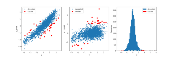
plt.figure(figsize=(15,5)) # 数据可视化 真实值预测值散点图
ax_131 = plt.subplot(1,3,1)
plt.plot(y,y_pred,'.')
plt.plot(y.loc[outliers],y_pred.loc[outliers],'ro')
plt.legend(['Accepted','Outlier'])
plt.xlabel('y')
plt.ylabel('y_pred');
ax_132=plt.subplot(1,3,2) # 真实值和残差散点图
plt.plot(y,y-y_pred,'.')
plt.plot(y.loc[outliers],y.loc[outliers]-y_pred.loc[outliers],'ro')
plt.legend(['Accepted','Outlier'])
plt.xlabel('y')
plt.ylabel('y - y_pred');
ax_133=plt.subplot(1,3,3) # 直方图
z.plot.hist(bins=50,ax=ax_133)
z.loc[outliers].plot.hist(color='r',bins=50,ax=ax_133)
plt.legend(['Accepted','Outlier'])
plt.xlabel('z')
plt.savefig('outliers.png',dpi = 200)
return outliers
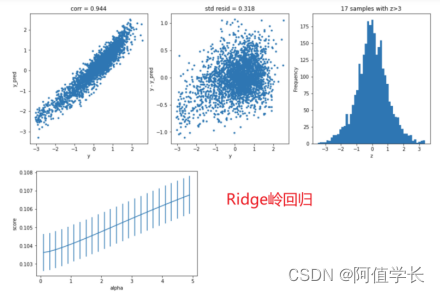
2.6.1 异常值检测-岭回归算法
from sklearn.linear_model import Ridge  # 获取训练数据
X_train, y_train = get_train_data()
outliers1 = find_outliers(Ridge(), X_train, y_train)  # 岭回归查找异常值
R2= 0.8689413869517439
mse= 0.12684550410078863
---------------------------------------
mean of residuals: -6.12198811189599e-17
std of residuals: 0.3562154416751183
---------------------------------------
30 outliers:
[348, 884, 1046, 1069, 1145, 1164, 1310, 1458, 1493, 1523, 1530, 1704, 1874, 2002, 2159, 2160, 2279, 2528, 2620, 2645, 2647, 2667, 2668, 2669, 2696, 2697, 2769, 2807, 2842, 2863]
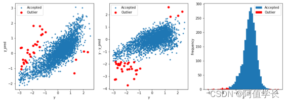
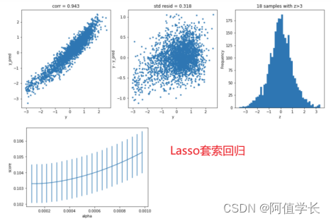
2.6.2 异常值检测-套索回归算法
from sklearn.linear_model import Lasso  # 获取训练数据
X_train, y_train = get_train_data()
outliers2 = find_outliers(Lasso(), X_train, y_train)  # 岭回归查找异常值
R2= 0.6220218641738002
mse= 0.3658273658084361
---------------------------------------
mean of residuals: 4.507397840626718e-16
std of residuals: 0.6049413865908968
---------------------------------------
31 outliers:
[332, 343, 376, 430, 884, 1064, 1065, 1126, 1311, 1365, 1442, 1477, 1828, 1874, 1932, 2030, 2253, 2254, 2255, 2256, 2257, 2279, 2281, 2579, 2580, 2581, 2636, 2663, 2667, 2790, 2807]
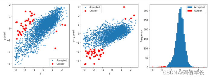
2.6.3 异常值检测-支持向量机SVR算法
from sklearn.svm import SVR  # 获取训练数据
X_train, y_train = get_train_data()
outliers3 = find_outliers(SVR(), X_train, y_train)  #  SVR查找异常值
R2= 0.6631924753676881
mse= 0.3259802561102477
---------------------------------------
mean of residuals: -0.04418097158794616
std of residuals: 0.5693334127618963
---------------------------------------
39 outliers:
[332, 343, 376, 884, 1064, 1065, 1126, 1138, 1311, 1365, 1442, 1477, 1828, 1874, 1932, 2030, 2161, 2253, 2254, 2255, 2256, 2257, 2264, 2279, 2281, 2334, 2339, 2579, 2580, 2581, 2620, 2635, 2636, 2637, 2645, 2663, 2667, 2790, 2807]
2.6.4 异常值检测-Xgboost算法
from xgboost import XGBRegressor  # 获取训练数据
X_train, y_train = get_train_data()
outliers4 = find_outliers(XGBRegressor(), X_train, y_train)  # 使用岭回归查找异常值
R2= 0.997493869079832
mse= 0.0024255669468609044
---------------------------------------
mean of residuals: 6.8967232026446646e-06
std of residuals: 0.04925857354764189
---------------------------------------
45 outliers:
[82, 124, 155, 178, 204, 293, 303, 577, 584, 620, 621, 641, 642, 674, 676, 722, 805, 846, 847, 1372, 1433, 1530, 1707, 1874, 1878, 1950, 1972, 1973, 1981, 2003, 2025, 2098, 2099, 2172, 2189, 2211, 2393, 2556, 2669, 2670, 2683, 2687, 2696, 2718, 2876]
2.6.5 异常值过滤
outliers12 = np.union1d(outliers1,outliers2)
outliers34 = np.union1d(outliers3,outliers4)
outliers = np.union1d(outliers12,outliers34)
display(outliers)
all_data = all_data.drop(labels=outliers)  # 过滤异常值
all_data.to_csv('./processed_zhengqi_data2.csv',index=False)
all_data.shape
array([  82,  124,  155,  178,  204,  293,  303,  332,  343,  348,  376,
        430,  577,  584,  620,  621,  641,  642,  674,  676,  722,  805,
...
       2528, 2556, 2579, 2580, 2581, 2620, 2635, 2636, 2637, 2645, 2647,
       2663, 2667, 2668, 2669, 2670, 2683, 2687, 2696, 2697, 2718, 2769,
       2790, 2807, 2842, 2863, 2876], dtype=int64)
(4709, 27)
2.7 多重共线性
2.7.1 多重共线性
指各特征之间存在线性相关关系,即一个特征可以是其他一个或几个特征的线性组合。如果存在多重共线性,求损失函数时矩阵不可逆,导致求出结果会与实际不同、有偏差,进行回归时影响系数准确性,就是多个特征存在线性关系,数据冗余但不完全,所以要将成线性关系的特征进行降维
2.7.2 多重共线性影响
(1) 变量之间高度相关时可能会给回归的结果造成混乱,甚至会把分析引入歧途
(2) 参数的含义不明确
(3) 变量的显著性检验失去意义,可能将重要的解释变量排除在模型之外
(4) 可使得本来不重要变量回归系数估计得很大或者重要变量回归系数估计得很小,从而产生错误判断
(5) 模型预测功能失效:变大的方差容易使预测区间变大,使预测失去意义
(6) 多重共线性影响的是模型系数确定性、解释性,就是线性回归模型的系数没有训练准确
2.7.3 多重共线性检验方法
方差膨胀系数(VIF):通常情况下,当VIF<10说明不存在多重共线性;当10<=VIF<100存在较强的多重共线性,当VIF >= 100存在严重多重共线性。方差膨胀系数原理:方差膨胀系数是衡量多元线性回归模型中多重共线性严重程度的一种度量。它表示回归系数估计量方差与假设自变量间不线性相关方差相比的比值
2.7.4 方差膨胀系数
from statsmodels.stats.outliers_influence import variance_inflation_factor # 方差膨胀系数
X_train,y_train = get_train_data()  # 多重共线性
X_train = np.matrix(X_train)
VIF_list=[round(variance_inflation_factor(X_train, i),2) for i in range(X_train.shape[1])]
print(VIF_list)
[110.83, 105.23, 78.58, 18.48, 153.54, 129.92, 69.49, 158.33, 59.58, 113.25, 15.1, 186.1, 84.68, 13.49, 12.8, 42.74, 36.63, 4.89, 121.61, 234.16, 12.55, 76.2, 39.29, 53.41, 38.4]
X_train.shape
(2784, 25)
2.7.5 PCA降维
from sklearn.decomposition import PCA
pca = PCA(n_components = 22,whiten=True)
X_train,y_train = get_train_data()
X_train_pca = np.matrix(pca.fit_transform(X_train))
VIF_pca_list=[round(variance_inflation_factor(X_train_pca, i),2) for i in range(X_train_pca.shape[1])]
print(VIF_pca_list)
np.savez('./train_data_pca',X_train = X_train_pca,y_train = y_train)
[1.0, 1.0, 1.0, 1.0, 1.0, 1.0, 1.0, 1.0, 1.0, 1.0, 1.0, 1.0, 1.0, 1.0, 1.0, 1.0, 1.0, 1.0, 1.0, 1.0, 1.0, 1.0]

X_test = get_test_data()
X_test_pca = pca.transform(X_test)
display(X_test_pca)
np.savez('./test_data_pca',X_test = X_test_pca)
array([[-4.10369816e-01, -1.07256951e-01, -4.28225234e-01, ...,
         4.49496885e-01,  2.42069040e-01,  5.45925385e-01],
       [-3.42908432e-01,  2.40043254e-01, -3.75608332e-01, ...,
        -2.11354338e-01,  4.13076485e-01,  6.94251955e-01],
       [-8.37774875e-01,  9.51729523e-01, -3.57728175e-01, ...,
        -8.80413195e-04,  6.74195344e-01,  1.13156001e+00],
       ...,
       [-3.09477429e+00, -5.92746365e-01, -1.13986964e+00, ...,
        -4.48546831e-01, -1.04121840e-01,  4.79249536e-02],
       [-3.01926790e+00, -6.20882854e-01, -1.15546927e+00, ...,
         1.01244969e-01,  2.54477699e-01, -7.73055486e-02],
       [-2.92817016e+00, -7.27309941e-01, -1.16525185e+00, ...,
         2.05687732e-01, -1.29672941e+00,  2.12695596e+00]])
2.8 模型初验
2.8.1 导库
from sklearn.linear_model import LinearRegression     # 线性回归
from sklearn.neighbors import KNeighborsRegressor    # K近邻回归
from sklearn.tree import DecisionTreeRegressor        # 决策树回归
from sklearn.ensemble import RandomForestRegressor  # 随机森林回归
from sklearn.svm import SVR                         #支持向量回归
import lightgbm as lgb                                # lightGbm模型
from sklearn.ensemble import GradientBoostingRegressor
from sklearn.model_selection import train_test_split  # 切分数据
from sklearn.metrics import mean_squared_error  #评价指标
2.8.2 数据拆分
train_data = np.load('./train_data_pca.npz')['X_train'] # 采用pca保留16维特征的数据
target_data = np.load('./train_data_pca.npz')['y_train']
X_train,X_valid,y_train,y_valid=train_test_split(train_data,target_data,test_size=0.2)
2.8.3 多元线性回归模型
clf = LinearRegression()
clf.fit(X_train, y_train)
score = mean_squared_error(y_valid, clf.predict(X_valid)) # 均方误差
print("LinearRegression:   ", score)
LinearRegression:    0.09534572535876486
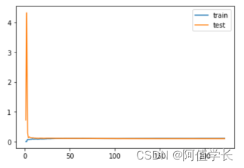
2.8.4 评估可视化
def plot_learning_curve(model, X_train, X_valid, y_train, y_valid):
    train_score = []
    valid_score = []
    for i in range(10, len(X_train)+1, 10):
        model.fit(X_train[:i], y_train[:i])
        y_train_predict = model.predict(X_train[:i])  # 训练数据评估
        train_score.append(mean_squared_error(y_train[:i], y_train_predict))
        y_valid_predict = model.predict(X_valid)  # 验证数据评估
        valid_score.append(mean_squared_error(y_valid, y_valid_predict))
    plt.plot([i for i in range(1, len(train_score)+1)],
            train_score, label="train")
    plt.plot([i for i in range(1, len(valid_score)+1)],
            valid_score, label="test")
    plt.legend()
plot_learning_curve(LinearRegression(), X_train, X_valid, y_train, y_valid)
plt.savefig('./9-多元线性回归训练验证数据评估对比.png',dpi = 200)
2.8.5 K近邻算法
for i in range(3,20):
    clf = KNeighborsRegressor(n_neighbors=i) # 最近三个
    clf.fit(X_train, y_train)
    score = mean_squared_error(y_valid, clf.predict(X_valid))
    print("KNeighborsRegressor:   ", score)
KNeighborsRegressor:    0.26255969220027925
KNeighborsRegressor:    0.2548952093806104
...
KNeighborsRegressor:    0.23830121017576525
KNeighborsRegressor:    0.24191366260188885
2.8.6 决策树回归
clf = DecisionTreeRegressor()
clf.fit(X_train, y_train)
score = mean_squared_error(y_valid, clf.predict(X_valid))
print("DecisionTreeRegressor:   ", score)
DecisionTreeRegressor:    0.30909928186714547
2.8.7 随机森林
clf = RandomForestRegressor(n_estimators=200,  # 200棵树模型
                            max_depth= 10,
                            max_features = 'auto', # 构建树时,特征筛选量
                            min_samples_leaf=10, # 是叶节点所需的最小样本数
                            min_samples_split=40, # 是分割所需的最小样本数
                            criterion='squared_error')
clf.fit(X_train, y_train)
score = mean_squared_error(y_valid, clf.predict(X_valid))
print("RandomForestRegressor:   ", score)
RandomForestRegressor:    0.1468589091112546
clf = RandomForestRegressor(n_estimators=200,  # 200棵树模型
                            max_depth= 10,
                            max_features = 'auto', # 构建树时,特征筛选量
                            min_samples_leaf=10, # 是叶节点所需的最小样本数
                            min_samples_split=40, # 是分割所需的最小样本数
                            criterion='squared_error')
plot_learning_curve(clf, X_train, X_valid, y_train, y_valid)

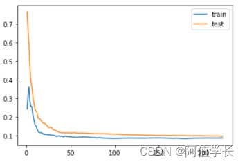
2.8.8 SVR支持向量机
(1) 错误项惩罚系数C:C越大即对分错样本惩罚程度越大,在训练样本中准确率越高但泛化能力降低;相反减小C容许训练样本中有一些误分类错误样本,泛化能力强。对于训练样本带有噪声情况,一般采用后者把训练样本集中错误分类的样本作为噪声
(2 )核函数系数gamma:rbf、poly和sigmoid核函数系数
(3) 分类容忍度epsilon:
 -用来定义模型对于错误分类容忍度,即错误分类而不受惩罚
 -epsilon值越大模型允许错误分类的容忍度越高,反之容忍度越小
 -支持向量的个数对epsilon大小敏感,即epsilon值越大支持向量个数越少,反之支持向量的个数越多
 -也可理解为epsilon值越小模型越过拟合,反之越大越欠拟合
clf1 = SVR(kernel='rbf',C = 1,gamma=0.01,tol = 0.0001,epsilon=0.3)
clf1.fit(X_train, y_train)
score = mean_squared_error(y_valid, clf1.predict(X_valid))
print("支持向量机高斯核函数:   ", score)
clf2 = SVR(kernel='poly')
clf2.fit(X_train, y_train)
score = mean_squared_error(y_valid, clf2.predict(X_valid))
print("支持向量机多项式核函数:   ", score)
支持向量机高斯核函数:    0.09761263112001187
支持向量机多项式核函数:    0.30199718825335975
plot_learning_curve(clf1,X_train, X_valid, y_train, y_valid)
2.8.9 lightGBM
(1) min_child_samples:一个叶子上最小数量。默认20。根据数据量来确定,当数据量比较大时应提升数值,让叶子节点数据分布相对稳定,提高模型泛化能力
(2) max_depth:树模型最大深度。防止过拟合最重要参数,一般限制为3~5之间。是需要调整的核心参数,对模型性能和泛化能力有决定性作用
(3) num_leaves:一棵树叶子节点个数。默认31,和max_depth配合来空值树的形状,一般设置(0, 2^max_depth - 1]一个数值。是需要重点调节参数,对模型性能影响很大
(4) L1正则化参数reg_alpha:别名lambda_l1默认0。这个参数不会有特别大差异,如发现这个参数数值大,则说明有一些没有太大作用的特征在模型内。需要调节来控制过拟合
(5) L2正则化参数reg_lambda:别名lambda_l2默认0。较大数值会让各个特征对模型影响力趋于均匀,不会有单个特征把持整个模型的表现。需要调节来控制过拟合
clf = lgb.LGBMRegressor(learning_rate=0.05,  # 学习率
                        n_estimators=300, # 集成树数量
                        min_child_samples=10, # 是叶节点所需的最小样本数
                        max_depth=5,  # 决策树深度
                        num_leaves = 25,
                        colsample_bytree =0.8, #构建树时特征选择比例
                        subsample=0.8, # 抽样比例
                        reg_alpha = 0.5,
                        reg_lambda = 0.1 )
clf.fit(X_train, y_train)
score = mean_squared_error(y_valid, clf.predict(X_valid))
print("LGB模型均方误差:   ", score)
LGB模型均方误差:    0.10153860165148278
2.8.10 GBDT
(1) min_sample_split :如果min_sample_split = 6并且节点中有4个样本,则不会发生拆分(不管熵是多少);假设min_sample_leaf = 3并且一个含有5个样本的节点可分别分裂成2个和3个大小的叶子节点,那这个分裂就不会发生,因为最小叶子大小为3
(2) 损失函数loss:
squared_error:均方误差
absolute_error:绝对损失
huber:上面两者融合
clf = GradientBoostingRegressor(learning_rate=0.03, # 学习率
loss='huber', # 损失函数
max_depth=14, # 决策树深度
max_features='sqrt', # 节点分裂时参与判断的最大特征数
min_samples_leaf=10, # 是叶节点所需的最小样本数
min_samples_split=40, # 是分割所需的最小样本数
n_estimators=300, # 集成树数量
subsample=0.8) # 抽样比例
clf.fit(X_train, y_train)
score = mean_squared_error(y_valid, clf.predict(X_valid))
print("GradientBoostingRegressor: ", score)
GradientBoostingRegressor: 0.09975389216573424
2.8.11 结论
(1) K近邻算法、决策树回归表现比较差
(2) 多元线性回归有待后续继续验证 (存在过拟合情况)
3.天池工业蒸汽量-模型预测
3.1 导库
import numpy as np
import pandas as pd
import matplotlib.pyplot as plt
from sklearn.linear_model import LinearRegression  # 线性回归
from sklearn.ensemble import RandomForestRegressor # 随机森林回归
from sklearn.ensemble import GradientBoostingRegressor
from sklearn.svm import SVR  # 支持向量回归
import lightgbm as lgb  # lightGbm模型
from xgboost import XGBRFRegressor
from sklearn.model_selection import train_test_split # 切分数据
from sklearn.metrics import mean_squared_error  # 评价指标
from sklearn.model_selection import learning_curve
from sklearn.model_selection import ShuffleSplit
import warnings
warnings.filterwarnings('ignore')
3.2 数据加载
3.2.1 未降维数据
all_data = pd.read_csv('./processed_zhengqi_data2.csv')
cond = all_data['label'] == 'train'
train_data = all_data[cond]
train_data.drop(labels = 'label',axis = 1,inplace = True)
X_train,X_valid,y_train,y_valid=train_test_split(train_data.drop(labels='target',axis = 1),train_data['target'],
                                                 test_size=0.2)
cond2 = all_data['label'] == 'test'
test_data = all_data[cond2]
test_data.drop(labels = ['label','target'],axis = 1,inplace = True)
all_data
3.2.2 降维数据
train_data_pca = np.load('./train_data_pca.npz')['X_train'] # 采用pca保留特征的数据
target_data_pca = np.load('./train_data_pca.npz')['y_train']
X_train_pca,X_valid_pca,y_train_pca,y_valid_pca=train_test_split(train_data_pca,target_data_pca,test_size=0.2)
test_data_pca = np.load('./test_data_pca.npz')['X_test']
train_data_pca.shape
(2784, 22)
3.3 学习曲线函数
def plot_learning_curve(model,title,X,y,cv=None):
    train_sizes, train_scores, test_scores = learning_curve(model, X, y, cv=cv)  # 学习曲线计算
    print(train_sizes,train_scores.shape,test_scores.shape)
    train_scores_mean = np.mean(train_scores, axis=1) # 训练数据得分和测试数据得分平均值与方差计算
    train_scores_std = np.std(train_scores, axis=1)
    test_scores_mean = np.mean(test_scores, axis=1)
    test_scores_std = np.std(test_scores, axis=1)
    plt.plot(train_sizes, train_scores_mean, 'o-', color="r",label="Training score")
    plt.fill_between(train_sizes, train_scores_mean - train_scores_std,
                     train_scores_mean + train_scores_std, alpha=0.1,color="r")
    plt.plot(train_sizes, test_scores_mean, 'o-', color="g",label="Cross-validation score")
    plt.fill_between(train_sizes, test_scores_mean - test_scores_std,
                     test_scores_mean + test_scores_std, alpha=0.1, color="g")
    plt.grid()  # 网格线设置
    plt.legend(loc="best")  # 图例设置
    plt.title(title)  # 标题标签设置
    plt.xlabel("Training examples")
    plt.ylabel("Score")
3.4 多元线性回归模型
3.4.1 模型训练
#(1) 降维数据建模验证
clf = LinearRegression()
clf.fit(X_train_pca, y_train_pca)
score = mean_squared_error(y_valid_pca, clf.predict(X_valid_pca))
print("LinearRegression:   ", score)
LinearRegression:    0.09376599064253983

#(2) 未降维数据建模验证
clf = LinearRegression()
clf.fit(X_train, y_train)
score = mean_squared_error(y_valid, clf.predict(X_valid))
print("LinearRegression:   ", score)
LinearRegression:    0.09754908135995455
3.4.2 绘制学习曲线
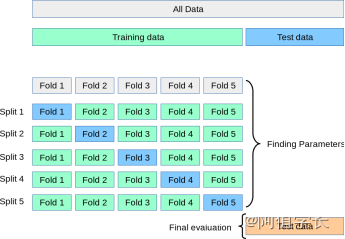
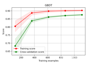
学习曲线是不同训练集大小模型在训练集和验证集上的得分变化曲线。以样本数为横坐标,训练和交叉验证集上的得分(如准确率)为纵坐标。learning curve可帮助判断模型现在所处状态:
过拟合(overfiting / high variance高方差)说明模型能很好拟合已知数据,但泛化能力很差属于高方差
欠拟合(underfitting / high bias 高偏差)说明模拟对已知数据和未知都不能进行准确预测,属于高偏差
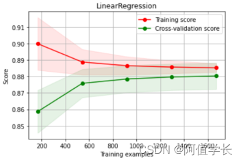
#(1) 降维数据学习曲线
X = X_train_pca
y = y_train_pca
title = "LinearRegression" # 多元线性回归模型学习曲线图
cv = ShuffleSplit(n_splits=100, test_size=0.25)
estimator = LinearRegression() # 建模
plot_learning_curve(estimator, title, X, y, cv = cv)
plt.savefig('./10-多元线性回归降维数据学习曲线.png',dpi = 200)
[ 167 542 918 1294 1670] (5, 100) (5, 100)
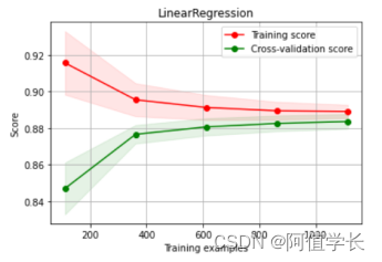
#(2) 非降维数据学习曲线
X = X_train
y = y_train
title = "LinearRegression"  # 多元线性回归模型学习曲线图
cv = ShuffleSplit(n_splits=100, test_size=0.5)
estimator = LinearRegression()    # 建模
plot_learning_curve(estimator, title, X, y, cv = cv)
plt.savefig('./11-多元线性回归非降维数据学习曲线.png',dpi = 200)
[ 111  361  612  862 1113] (5, 100) (5, 100)
3.4.3  降维数据建模预测提交
model = LinearRegression()  # 得分是:0.1598
model.fit(train_data_pca,target_data_pca)
y_ = model.predict(test_data_pca)
display(y_)
np.savetxt('./多元线性回归模型预测(降维数据).txt',y_)
array([ 0.18802274,  0.24611291, -0.1557421 , ..., -2.46741335,
       -2.51810503, -2.23076209])

3.4.4  非降维数据建模预测提交
model = LinearRegression()  # 得分是:0.1620
model.fit(train_data.drop('target',axis = 1),train_data['target'])
y_ = model.predict(test_data)
display(y_)
np.savetxt('./多元线性回归模型预测(非降维数据).txt',y_)
array([ 0.180302  ,  0.21599399, -0.17268982, ..., -2.44517796,
       -2.44884392, -2.06587572])

3.5 随机森林模型
3.5.1 模型训练
#(1) 降维数据建模验证
model = RandomForestRegressor(n_estimators=200, # 200棵树模型
                            max_depth= 10,
                            max_features = 'auto',  # 构建树时,特征筛选量
                            min_samples_leaf=10,  # 是叶节点所需的最小样本数
                            min_samples_split=40,  # 是分割所需的最小样本数
                            criterion='squared_error')
model.fit(X_train_pca, y_train_pca)
score = mean_squared_error(y_valid_pca, model.predict(X_valid_pca))
print("随机森林得分:   ", score)
随机森林得分:    0.1535330953946485

#(2) 非降维数据建模验证
model = RandomForestRegressor(n_estimators=200,  # 200棵树模型
                            max_depth= 10,
                            max_features = 'auto', # 构建树时,特征筛选量
                            min_samples_leaf=10, # 是叶节点所需的最小样本数
                            min_samples_split=40, # 是分割所需的最小样本数
                            criterion='squared_error')
model.fit(X_train, y_train)
score = mean_squared_error(y_valid, model.predict(X_valid))
print("随机森林得分:   ", score)
随机森林得分:    0.10046589910006855
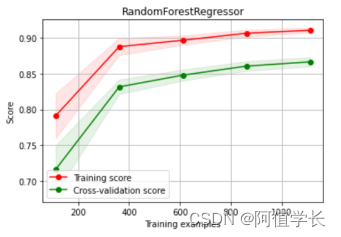
3.5.2 绘制学习曲线
%%time
X = X_train
y = y_train
title = "RandomForestRegressor"  # 随机森林模型学习曲线图
cv = ShuffleSplit(n_splits=100, test_size=0.5)
model = RandomForestRegressor(n_estimators=200,  # 200棵树模型
                            max_depth= 10,
                            max_features = 'auto', # 构建树时,特征筛选量
                            min_samples_leaf=10, # 是叶节点所需的最小样本数
                            min_samples_split=40, # 是分割所需的最小样本数
                            criterion='squared_error')
plot_learning_curve(model, title, X, y, cv = cv)
plt.savefig('./12-随机森林非降维数据学习曲线.png',dpi = 200)
[ 111  361  612  862 1113] (5, 100) (5, 100)
Wall time: 4min 53s
3.5.3 模型预测
#(1) 降维数据建模预测提交  得分是:1.0579
model =  RandomForestRegressor(n_estimators=200, # 200棵树模型
                            max_depth= 10,
                            max_features = 'auto', # 构建树时,特征筛选量
                            min_samples_leaf=10, # 是叶节点所需的最小样本数
                            min_samples_split=40, # 是分割所需的最小样本数
                            criterion='squared_error')
model.fit(train_data_pca,target_data_pca)
y_ = model.predict(test_data_pca)
display(y_)
np.savetxt('./随机森林模型预测(降维数据).txt',y_)
array([ 0.31543138,  0.23577324, -0.18489794, ..., -2.39873726,
       -2.41017305, -2.31572213])

#(2) 非降维数据建模预测提交 得分是:0.1461
model = RandomForestRegressor(n_estimators=200, # 200棵树模型
                            max_depth= 10,
                            max_features = 'auto',# 构建树时,特征筛选量
                            min_samples_leaf=10,# 是叶节点所需的最小样本数
                            min_samples_split=40,# 是分割所需的最小样本数
                            criterion='squared_error')
model.fit(train_data.drop('target',axis = 1),train_data['target'])
y_ = model.predict(test_data)
display(y_)
np.savetxt('./随机森林模型预测(非降维数据).txt',y_)
array([ 0.31188585,  0.18338938, -0.085748  , ..., -2.65705188,
       -2.65935435, -2.65767658])

3.6 SVR支持向量机
3.6.1 模型训练
#(1) 降维数据
model = SVR(kernel='rbf',C = 1,gamma=0.01,tol = 0.0001,epsilon=0.3)
model.fit(X_train_pca, y_train_pca)
score = mean_squared_error(y_valid_pca, model.predict(X_valid_pca))
print("SVR支持向量机得分:   ", score)
SVR支持向量机得分:    0.09631380213015923
#(2) 非降维数据
model = SVR(kernel='rbf')
model.fit(X_train, y_train)
score = mean_squared_error(y_valid, model.predict(X_valid))
print("SVR支持向量机得分:   ", score)
SVR支持向量机得分:    0.25202455384213157
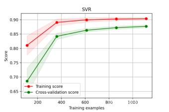
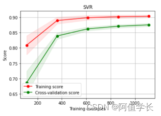
3.6.2 绘制学习曲线
#(1) 降维数据
%%time
X = X_train_pca
y = y_train_pca
title = "SVR"  # 随机森林模型学习曲线图
cv = ShuffleSplit(n_splits=100, test_size=0.5)
model = SVR(kernel='rbf',C = 1,gamma=0.01,tol = 0.0001,epsilon=0.3)
plot_learning_curve(model, title, X, y, cv = cv)
plt.savefig('./15-SVR降维数据学习曲线.png',dpi = 200)
[ 111  361  612  862 1113] (5, 100) (5, 100)
Wall time: 22.5 s
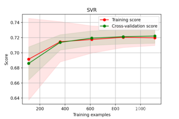
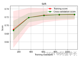
#(2) 非降维数据
%%time
X = X_train
y = y_train
title = "SVR"  # 随机森林模型学习曲线图
cv = ShuffleSplit(n_splits=100, test_size=0.5)
model = SVR(kernel='rbf')
plot_learning_curve(model, title, X, y, cv = cv)
plt.savefig('./16-SVR非降维数据学习曲线.png',dpi = 200)
[ 111  361  612  862 1113] (5, 100) (5, 100)
Wall time: 53.6 s
3.6.3 SVR模型预测
#(1) 降维数据  得分是:0.2654
model = SVR(kernel='rbf',C = 1,gamma=0.01,tol = 0.0001,epsilon=0.3)
model.fit(train_data_pca,target_data_pca)
y_ = model.predict(test_data_pca)
display(y_)
np.savetxt('./SVR模型预测(降维数据).txt',y_)
array([ 0.26958642,  0.25920386, -0.10122391, ..., -2.22155225,
       -2.3239961 , -2.18865886])

#(2) 非降维数据  得分是:1.9934
model =SVR(kernel='rbf')
model.fit(train_data.drop('target',axis = 1),train_data['target'])
y_ = model.predict(test_data)
display(y_)
np.savetxt('./SVR模型预测(非降维数据).txt',y_)
array([ 0.02366046,  0.0795185 , -0.3815812 , ..., -3.27797957,
       -3.20270896, -3.10625782])

#(3) poly多项式核函数建模预测--降维数据  得分是:4.7068
model = SVR(kernel='poly')
model.fit(train_data_pca,target_data_pca)
y_ = model.predict(test_data_pca)
display(y_)
np.savetxt('./SVR-poly模型预测(降维数据).txt',y_)
array([ 0.20042313,  0.26680596,  0.14459824, ..., -4.66039099,
       -3.79414397, -2.76923448])

#(4) poly多项式核函数建模预测--非降维数据  得分是:0.7423
model =SVR(kernel='poly')
model.fit(train_data.drop('target',axis = 1),train_data['target'])
y_ = model.predict(test_data)
display(y_)
np.savetxt('./SVR--poly模型预测(非降维数据).txt',y_)
array([-0.07224459, -0.04512705, -0.21601474, ..., -0.45687101,
       -0.45655309, -0.45593334])


3.7 GBDT梯度提升树
3.7.1 模型训练
#(1) 降维数据
model = GradientBoostingRegressor(learning_rate=0.03, # 学习率
                                loss='huber',  # 损失函数
                                max_depth=14, # 决策树深度
                                max_features='sqrt',# 节点分裂时参与判断的最大特征数
                                min_samples_leaf=10,# 是叶节点所需的最小样本数
                                min_samples_split=40,# 是分割所需的最小样本数
                                n_estimators=300,# 集成树数量
                                subsample=0.8)# 抽样比例
model.fit(X_train_pca, y_train_pca)
score = mean_squared_error(y_valid_pca, model.predict(X_valid_pca))
print("GBDT得分:   ", score)
GBDT得分:    0.1052596997571393

#(2) 非降维数据
model = GradientBoostingRegressor(learning_rate=0.03, # 学习率
                                loss='huber',  # 损失函数
                                max_depth=14, # 决策树深度
                                max_features='sqrt',# 节点分裂时参与判断的最大特征数
                                min_samples_leaf=10,# 是叶节点所需的最小样本数
                                min_samples_split=40,# 是分割所需的最小样本数
                                n_estimators=300,# 集成树数量
                                subsample=0.8)# 抽样比例
model.fit(X_train, y_train)
score = mean_squared_error(y_valid, model.predict(X_valid))
print("GBDT得分:   ", score)
GBDT得分:    0.1052596997571393
3.7.2 绘制学习曲线
#(1) 降维数据学习曲线
%%time
X = X_train_pca
y = y_train_pca
title = "GBDT"  # 随机森林模型学习曲线图
cv = ShuffleSplit(n_splits=100, test_size=0.5)
model = GradientBoostingRegressor(learning_rate=0.03, # 学习率
                                loss='huber',  # 损失函数
                                max_depth=14, # 决策树深度
                                max_features='sqrt',# 节点分裂时参与判断的最大特征数
                                min_samples_leaf=10,# 是叶节点所需的最小样本数
                                min_samples_split=40,# 是分割所需的最小样本数
                                n_estimators=300,# 集成树数量
                                subsample=0.8)# 抽样比例
plot_learning_curve(model, title, X, y, cv = cv)
plt.savefig('./17-GBDT降维数据学习曲线.png',dpi = 200)
3.7.3 模型预测
#(1) 降维数据  得分是:0.3765
model =  GradientBoostingRegressor(learning_rate=0.03, # 学习率
                                loss='huber',  # 损失函数
                                max_depth=14, # 决策树深度
                                max_features='sqrt', # 节点分裂时参与判断的最大特征数
                                min_samples_leaf=10, # 是叶节点所需的最小样本数
                                min_samples_split=40, # 是分割所需的最小样本数
                                n_estimators=300, # 集成树数量
                                subsample=0.8) # 抽样比例
model.fit(train_data_pca,target_data_pca)
y_ = model.predict(test_data_pca)
display(y_)
np.savetxt('./GBDT模型预测(降维数据).txt',y_)
array([ 0.39815808,  0.20234983,  0.08249647, ..., -1.77946695,
       -1.92080868, -1.89811382])

#(2) 非降维数据  得分是:0.1392
model = GradientBoostingRegressor(learning_rate=0.03, # 学习率
                                loss='huber',  # 损失函数
                                max_depth=14, # 决策树深度
                                max_features='sqrt',# 节点分裂时参与判断的最大特征数
                                min_samples_leaf=10,# 是叶节点所需的最小样本数
                                min_samples_split=40,# 是分割所需的最小样本数
                                n_estimators=300,# 集成树数量
                                subsample=0.8)# 抽样比例
model.fit(train_data.drop('target',axis = 1),train_data['target'])
y_ = model.predict(test_data)
display(y_)
np.savetxt('./GBDT模型预测(非降维数据).txt',y_)
array([ 4.45480904e-01,  3.03493216e-01, -2.65851462e-04, ...,
       -2.59291666e+00, -2.72350856e+00, -2.61891111e+00])

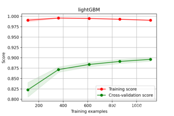
3.8 LightGBM轻量梯度提升模型
3.8.1 模型训练
#(1) 降维数据
model = lgb.LGBMRegressor(learning_rate=0.05, # 学习率
                        n_estimators=300,# 集成树数量
                        min_child_samples=10,# 是叶节点所需的最小样本数
                        max_depth=5, # 决策树深度
                        num_leaves = 25,
                        colsample_bytree =0.8,#构建树时特征选择比例
                        subsample=0.8,# 抽样比例
                        reg_alpha = 0.5,
                        reg_lambda = 0.1 )
model.fit(X_train_pca, y_train_pca)
score = mean_squared_error(y_valid_pca, model.predict(X_valid_pca))
print("LGB得分:   ", score)
LGB得分:    0.10182794462374979

#(2) 非降维数据
model = lgb.LGBMRegressor(learning_rate=0.05, # 学习率
                        n_estimators=300,# 集成树数量
                        min_child_samples=10,# 是叶节点所需的最小样本数
                        max_depth=5, # 决策树深度
                        num_leaves = 25,
                        colsample_bytree =0.8,#构建树时特征选择比例
                        subsample=0.8,# 抽样比例
                        reg_alpha = 0.5,
                        reg_lambda = 0.1 )
model.fit(X_train, y_train)
score = mean_squared_error(y_valid, model.predict(X_valid))
print("LGB得分:   ", score)
LGB得分:    0.10182794462374979
3.8.2 绘制学习曲线
#(1) 降维数据
%%time
X = X_train
y = y_train
title = "lightGBM"  #  lightGBM模型学习曲线图
cv = ShuffleSplit(n_splits=100, test_size=0.5)
model = lgb.LGBMRegressor(learning_rate=0.05, # 学习率
                        n_estimators=300,# 集成树数量
                        min_child_samples=10,# 是叶节点所需的最小样本数
                        max_depth=5, # 决策树深度
                        num_leaves = 25,
                        colsample_bytree =0.8,#构建树时特征选择比例
                        subsample=0.8,# 抽样比例
                        reg_alpha = 0.5,
                        reg_lambda = 0.1 )
plot_learning_curve(model, title, X, y, cv = cv)
plt.savefig('./22-lightGBM非降维数据学习曲线.png',dpi = 200)
[ 111  361  612  862 1113] (5, 100) (5, 100)
Wall time: 1min 17s
3.8.3 模型预测
#(1) 降维数据  得分是:0.6383
model =  lgb.LGBMRegressor(learning_rate=0.05, # 学习率
                        n_estimators=100,# 集成树数量
                        min_child_samples=10,# 是叶节点所需的最小样本数
                        max_depth=5, # 决策树深度
                        num_leaves = 25,
                        colsample_bytree =0.8,#构建树时特征选择比例
                        subsample=0.8,# 抽样比例
                        reg_alpha = 0.5,
                        reg_lambda = 0.1 )
model.fit(train_data_pca,target_data_pca)
y_ = model.predict(test_data_pca)
display(y_)
np.savetxt('./lightGBM模型预测(降维数据).txt',y_)
array([ 0.27629405,  0.26720862,  0.04551531, ..., -1.88494216,
       -2.03600739, -1.76903934])

#(2) 非降维数据  得分是:0.1378
model = lgb.LGBMRegressor(learning_rate=0.05, # 学习率
                        n_estimators=100,# 集成树数量
                        min_child_samples=10,# 是叶节点所需的最小样本数
                        max_depth=5, # 决策树深度
                        num_leaves = 25,
                        colsample_bytree =0.8,#构建树时特征选择比例
                        subsample=0.8,# 抽样比例
                        reg_alpha = 0.5,
                        reg_lambda = 0.1 )
model.fit(train_data.drop('target',axis = 1),train_data['target'])
y_ = model.predict(test_data)
display(y_)
np.savetxt('./lightGBM模型预测(非降维数据).txt',y_)
array([ 0.31735247,  0.21516006, -0.02321356, ..., -2.63261151,
       -2.64385024, -2.71366543])

3.9 Xgboost极限梯度提升树
3.9.1 模型训练
#(1) 降维数据
model = XGBRFRegressor(n_estimators = 300,
                       max_depth=15,
                       subsample = 0.8,
                       colsample_bytree = 0.8,
                       learning_rate =1,
                       gamma = 0,
                       reg_lambda= 0 ,  # L2正则化
                       reg_alpha = 0,verbosity=1)  # L1正则化
model.fit(X_train_pca, y_train_pca)
score = mean_squared_error(y_valid_pca, model.predict(X_valid_pca))
print("Xgboost得分:   ", score)
Xgboost得分:    0.13430091438485942

#(2) 非降维数据
model = XGBRFRegressor(n_estimators = 300,
                       max_depth=15,
                       subsample = 0.8,
                       colsample_bytree = 0.8,
                       learning_rate =1,
                       gamma = 0,
                       reg_lambda= 0 ,  # L2正则化
                       reg_alpha = 0,verbosity=1)  # L1正则化
model.fit(X_train, y_train)
score = mean_squared_error(y_valid, model.predict(X_valid))
print("Xgboost得分:   ", score)
Xgboost得分:    0.08908612728637443
3.9.2 Xgboost模型预测
#(1) 降维数据  得分是:0.6798
model = XGBRFRegressor(n_estimators = 300,
                       max_depth=15,
                       subsample = 0.8,
                       colsample_bytree = 0.8,
                       learning_rate =1,
                       gamma = 0,
                       reg_lambda= 0 ,  # L2正则化
                       reg_alpha = 0,verbosity=1)  # L1正则化
model.fit(train_data_pca,target_data_pca)
y_ = model.predict(test_data_pca)
display(y_)
np.savetxt('./Xgboost模型预测(降维数据).txt',y_)
array([ 0.39872065,  0.29756796,  0.06591171, ..., -1.8471452 ,
       -1.8405936 , -1.7466732 ], dtype=float32)

#(2) 非降维数据  得分是:0.1329
model = XGBRFRegressor(n_estimators = 300,
                       max_depth=15,
                       subsample = 0.8,
                       colsample_bytree = 0.8,
                       learning_rate =1,
                       gamma = 0,
                       reg_lambda= 0 ,  # L2正则化
                       reg_alpha = 0,verbosity=1)  # L1正则化
model.fit(train_data.drop('target',axis = 1),train_data['target'])
y_ = model.predict(test_data)
display(y_)
np.savetxt('./Xgboost模型预测(非降维数据).txt',y_)
array([ 0.38381824,  0.21534394, -0.04474839, ..., -2.7662156 ,
       -2.7820516 , -2.8380976 ], dtype=float32)

3.10 模型预测结论
(1) 集成算法对非降维数据表现更好
(2) 多元线性回归、SVR对降维数据表现更好
(3) 整体来说集成算法效果更好
(4) 随机森林:0.1461
(5) GBDT:0.1392
(6) lightGBM:0.1378
(7) Xgboost:0.1329
(8) 还需要继续对特征进行挖掘、对算法进行融合
4.天池工业蒸汽量-模型融合
4.1 导库
import numpy as np
import pandas as pd
import matplotlib.pyplot as plt
from sklearn.linear_model import Ridge,Lasso,ElasticNet  # 线性回归
from sklearn.ensemble import RandomForestRegressor # 随机森林回归
from sklearn.ensemble import GradientBoostingRegressor
from sklearn.svm import SVR  # 支持向量回归
import lightgbm as lgb   # lightGbm模型
from xgboost import XGBRFRegressor
from sklearn.model_selection import train_test_split  # 切分数据
from sklearn.metrics import mean_squared_error   # 评价指标
from sklearn.model_selection import RepeatedKFold
from sklearn.model_selection import GridSearchCV
import warnings
warnings.filterwarnings('ignore')
4.2 数据加载
4.2.1 特征工程(未降维数据)
all_data = pd.read_csv('./processed_zhengqi_data2.csv')
cond = all_data['label'] == 'train'  # 训练数据
train_data = all_data[cond]
train_data.drop(labels = 'label',axis = 1,inplace = True)
X = train_data.drop(labels='target',axis = 1)  # 从训练数据中提取特征数据X和目标值y
y = train_data['target']
X_train,X_valid,y_train,y_valid=train_test_split(X,y,test_size=0.2)  # 切分数据 训练数据80% 验证数据20%
cond2 = all_data['label'] == 'test'  # 测试提交数据
submit_test = all_data[cond2]
submit_test.drop(labels = ['label','target'],axis = 1,inplace = True)
4.2.2 特征工程(降维数据)
X_pca = np.load('./train_data_pca.npz')['X_train']  # 采用 pca 保留特征的数据
y_pca = np.load('./train_data_pca.npz')['y_train']
X_train_pca,X_valid_pca,y_train_pca,y_valid_pca=train_test_split(X_pca,y_pca, test_size=0.2)
submit_test_pca = np.load('./test_data_pca.npz')['X_test']
4.3 网格搜索调参
def train_model(model, param_grid=[], X=[], y=[],splits=5, repeats=5):
    rkfold = RepeatedKFold(n_splits=splits, n_repeats=repeats)  # 创建网格交叉
    gsearch = GridSearchCV(model, param_grid, cv=rkfold,scoring='neg_mean_squared_error',
                           verbose=1, return_train_score=True)  # 设置网格搜索参数
    gsearch.fit(X,y)  # 网格搜索训练
    model = gsearch.best_estimator_     # 提取最优算法
    best_idx = gsearch.best_index_      # 最优算法索引:获得最优算法平均得分和标准差
    grid_results = pd.DataFrame(gsearch.cv_results_)
    cv_mean = abs(grid_results.loc[best_idx,'mean_test_score'])
    cv_std = grid_results.loc[best_idx,'std_test_score']
    cv_score = pd.Series({'mean':cv_mean,'std':cv_std})  # 平均值和方差数据合并
    y_pred = model.predict(X)  # 预测
    print('----------------------')
    print(model)  # 输出模型评价指标
    print('----------------------')
    print('score=',model.score(X,y))
    print('mse=',mean_squared_error(y, y_pred))
    print('cross_val: mean=',cv_mean,', std=',cv_std)
    y_pred = pd.Series(y_pred,index=y.index)  # 残差数据可视化
    resid = y - y_pred
    mean_resid = resid.mean()
    std_resid = resid.std()
    z = (resid - mean_resid)/std_resid  # 残差标准化Z-score
    n_outliers = sum(abs(z)>3)
    plt.figure(figsize=(15,5))
    ax1 = plt.subplot(1,3,1)
    plt.plot(y,y_pred,'.')
    plt.xlabel('y')
    plt.ylabel('y_pred');
    plt.title('corr = {:.3f}'.format(np.corrcoef(y,y_pred)[0][1]))
    ax2=plt.subplot(1,3,2)
    plt.plot(y,y-y_pred,'.')
    plt.xlabel('y')
    plt.ylabel('y - y_pred');
    plt.title('std resid = {:.3f}'.format(std_resid))
    ax3=plt.subplot(1,3,3)
    z.plot.hist(bins=50,ax=ax3)
    plt.xlabel('z')
    plt.title('{:.0f} samples with z>3'.format(n_outliers))
    return model, cv_score, grid_results
4.4 非降维数据
opt_models = dict()  # 可选模型
score_models = pd.DataFrame(columns=['mean','std'])  # 记录模型表现
splits = 5
repeats = 5
4.4.1 Ridge岭回归
%%time
model = 'Ridge'
opt_models[model] = Ridge()
alphas = np.arange(0.1,5,0.2)
param_grid = {'alpha': alphas}
opt_models[model],cv_score,grid_results = train_model(opt_models[model],
                                                      param_grid=param_grid,
                                                      X = X,y = y,
                                                      splits=splits, repeats=repeats)
cv_score.name = model
score_models = score_models.append(cv_score)
plt.figure()
plt.errorbar(alphas, abs(grid_results['mean_test_score']),
             abs(grid_results['std_test_score'])/np.sqrt(splits*repeats))
plt.xlabel('alpha')
plt.ylabel('mse')
Fitting 25 folds for each of 25 candidates, totalling 625 fits
----------------------
Ridge(alpha=0.1)
----------------------
score= 0.8902000535130349
mse= 0.10092360225245812
cross_val: mean= 0.10336376761792092 , std= 0.005363070368960136
Wall time: 4.14 s
Text(0, 0.5, 'mse')
4.4.2 Lasso套索回归
%%time
model = 'Lasso'
opt_models[model] = Lasso()
alphas = np.arange(1e-4,1e-3,4e-5)
param_grid = {'alpha': alphas}
opt_models[model], cv_score, grid_results = train_model(opt_models[model],
                                                        param_grid=param_grid,
                                                        X = X,y = y,
                                                        splits=splits, repeats=repeats)
cv_score.name = model
score_models = score_models.append(cv_score)
plt.figure()
plt.errorbar(alphas, abs(grid_results['mean_test_score']),
             abs(grid_results['std_test_score'])/np.sqrt(splits*repeats))
plt.xlabel('alpha')
plt.ylabel('mse')
Fitting 25 folds for each of 23 candidates, totalling 575 fits
----------------------
Lasso(alpha=0.0001)
----------------------
score= 0.8901155559523605
mse= 0.10100126894062737
cross_val: mean= 0.10377223089437403 , std= 0.004806415049746983
Wall time: 10.6 s
Text(0, 0.5, 'mse')
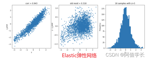
4.4.3 ElasticNet弹性网络
model ='ElasticNet'
opt_models[model] = ElasticNet(max_iter=10000)
param_grid = {'alpha': np.arange(1e-4,1e-3,1e-4),
              'l1_ratio': np.arange(0.1,1.0,0.1)}
opt_models[model], cv_score, grid_results = train_model(opt_models[model],
                                                        param_grid=param_grid,
                                                        X = X,y = y,
                                                        splits=splits, repeats=repeats)
cv_score.name = model
score_models = score_models.append(cv_score)
Fitting 25 folds for each of 81 candidates, totalling 2025 fits
----------------------
ElasticNet(alpha=0.0001, l1_ratio=0.30000000000000004, max_iter=10000)
----------------------
score= 0.8901312137886744
mse= 0.10098687690042292
cross_val: mean= 0.1037081857011029 , std= 0.0075442721802750036
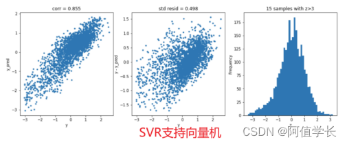
4.4.4 SVR支持向量机
%%time
model='SVR'
opt_models[model] = SVR()
param_grid = {'C':np.arange(0.1,1.0,0.2)}
opt_models[model], cv_score, grid_results = train_model(opt_models[model],
                                                        param_grid=param_grid,
                                                        X = X,y = y,
                                                        splits=splits, repeats=repeats)
cv_score.name = model
score_models = score_models.append(cv_score)
Fitting 25 folds for each of 5 candidates, totalling 125 fits
----------------------
SVR(C=0.9000000000000001)
----------------------
score= 0.7295322521443957
mse= 0.24860284799808752
cross_val: mean= 0.24932472306396555 , std= 0.010996974167330562
Wall time: 1min 7s
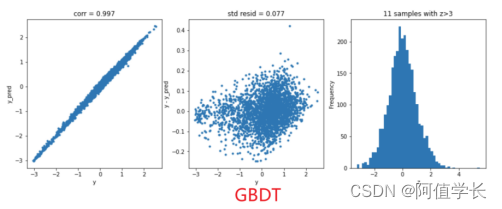
4.4.5 GBDT梯度提升回归树
%%time
model = 'GradientBoosting'
opt_models[model] = GradientBoostingRegressor()
param_grid = {'n_estimators':[100,200,300],
              'max_depth':[3,5,7],
              'min_samples_split':[5,6,7]}
opt_models[model], cv_score, grid_results = train_model(opt_models[model],
                                                        param_grid=param_grid,
                                                        X = X,y = y,
                                                        splits=splits, repeats=1)
cv_score.name = model
score_models = score_models.append(cv_score)
Fitting 5 folds for each of 27 candidates, totalling 135 fits
----------------------
GradientBoostingRegressor(max_depth=5, min_samples_split=5, n_estimators=200)
----------------------
score= 0.9881571826018469
mse= 0.01088543146768819
cross_val: mean= 0.08976167618394948 , std= 0.0022245830289117693
Wall time: 6min 54s
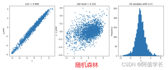
4.4.6 RFR随机森林
%%time
model = 'RandomForest'
opt_models[model] = RandomForestRegressor()
param_grid = {'n_estimators':[100,200,300],
              'max_features':[12,16,20,24],
              'min_samples_split':[5,7,9]}
opt_models[model], cv_score, grid_results = train_model(opt_models[model],
                                                        param_grid=param_grid,
                                                        X = X,y = y,
                                                        splits=splits, repeats=1)
cv_score.name = model
score_models = score_models.append(cv_score)
Fitting 5 folds for each of 36 candidates, totalling 180 fits
----------------------
RandomForestRegressor(max_features=16, min_samples_split=5, n_estimators=200)
----------------------
score= 0.9818017045248687
mse= 0.01672712595012877
cross_val: mean= 0.09554611688004881 , std= 0.006548665559568625
Wall time: 7min 53s
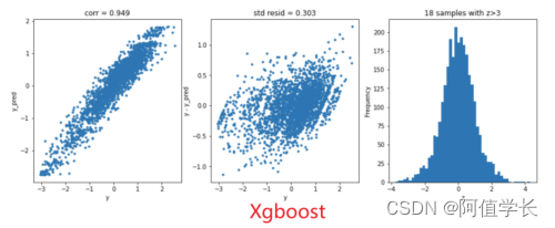
4.4.7 Xgboost极限梯度提升树
%%time
model = 'XGB'
opt_models[model] = XGBRFRegressor()
param_grid = {'n_estimators':[200,300],
              'max_depth':[3,5],
              'reg_lambda': np.arange(1e-5,1e-3,1e-4)}
opt_models[model], cv_score,grid_results = train_model(opt_models[model],
                                                        param_grid=param_grid,
                                                        X = X,y = y,
                                                        splits=splits, repeats=1)
cv_score.name = model
score_models = score_models.append(cv_score)
Fitting 5 folds for each of 40 candidates, totalling 200 fits
----------------------
XGBRFRegressor(base_score=0.5, booster='gbtree', colsample_bylevel=1,
               colsample_bytree=1, enable_categorical=False, gamma=0, gpu_id=-1,
               importance_type=None, interaction_constraints='',
               max_delta_step=0, max_depth=5, min_child_weight=1, missing=nan,
               monotone_constraints='()', n_estimators=300, n_jobs=16,
               num_parallel_tree=300, objective='reg:squarederror',
               predictor='auto', random_state=0, reg_alpha=0,
               reg_lambda=0.00021, scale_pos_weight=1, tree_method='exact',
               validate_parameters=1, verbosity=None)
----------------------
score= 0.9003007450187164
mse= 0.09163946137070277
cross_val: mean= 0.1164286657351558 , std= 0.005785578696726894
Wall time: 1min 31s
4.4.8 LightGBM轻量梯度提升模型
%%time
model = 'lightGBM'
opt_models[model] = lgb.LGBMRegressor()
param_grid = {'n_estimators':[200,300],
              'max_depth':[3,5],
              'min_child_weight': range(3, 6, 1),
              'reg_alpha': [1e-5, 1e-2, 0.1, 1],
              'reg_lambda': [1e-5, 1e-2, 0.1, 1]}
opt_models[model], cv_score,grid_results = train_model(opt_models[model],
                                                        param_grid=param_grid,
                                                        X = X,y = y,
                                                        splits=splits, repeats=1)
cv_score.name = model
score_models = score_models.append(cv_score)
Fitting 5 folds for each of 192 candidates, totalling 960 fits
----------------------
LGBMRegressor(max_depth=5, min_child_weight=3, n_estimators=200, reg_alpha=0.01,
              reg_lambda=0.01)
----------------------
score= 0.9791955891359189
mse= 0.019122560204457892
cross_val: mean= 0.08946762026703706 , std= 0.004600778509210142
Wall time: 2min 17s
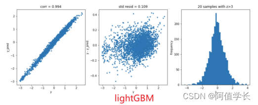
4.5 模型预测-多模型融合bagging
def model_predict(submit_test):
    i=0
    y_predict_total = np.zeros(submit_test.shape[0])
    for model in opt_models.keys():
        y_predict = opt_models[model].predict(submit_test)
        y_predict_total += y_predict
        i+=1
    y_predict_mean = np.round(y_predict_total/i,3)   # 求平均
    return y_predict_mean
4.6 预测结果提交
result = model_predict(submit_test)
np.savetxt('./bagging_result.txt',result)
result
array([ 0.251,  0.217, -0.122, ..., -2.674, -2.69 , -2.513])


 被折叠的 条评论
为什么被折叠?
被折叠的 条评论
为什么被折叠?
 到【灌水乐园】发言


