Kaggle比赛入门 - Titanic - Machine Learning from Disaster

导入packages，打印文件的路径

import numpy as np # linear algebra
import pandas as pd # data processing, CSV file I/O (e.g. pd.read_csv)
import seaborn as sns
import matplotlib.pyplot as plt

import os
for dirname, _, filenames in os.walk('/kaggle/input'):
    for filename in filenames:
        print(os.path.join(dirname, filename))

/kaggle/input/titanic/train.csv
/kaggle/input/titanic/test.csv
/kaggle/input/titanic/gender_submission.csv

读取train和test的数据

training = pd.read_csv('/kaggle/input/titanic/train.csv')
test = pd.read_csv('/kaggle/input/titanic/test.csv')

结合train和test的数据

training['train_test'] = 1
test['train_test'] = 0
test['Survived'] = np.NaN
all_data = pd.concat([training, test])

返回数据框的所有列名

%matplotlib inline 
all_data.columns

输出：

Index(['PassengerId', 'Survived', 'Pclass', 'Name', 'Sex', 'Age', 'SibSp',
       'Parch', 'Ticket', 'Fare', 'Cabin', 'Embarked', 'train_test'],
      dtype='object')

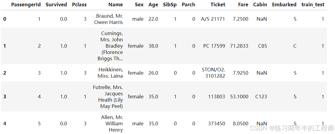
打印前5行的数据

all_data.head()

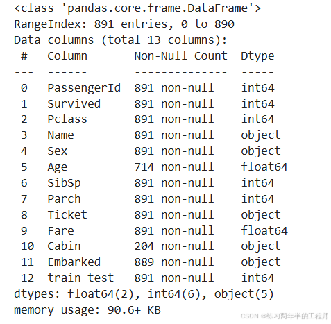
查看train的数据

# quick look at the data types & null counts
training.info()

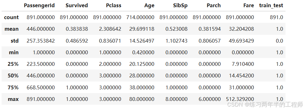
查看train的数据的统计资料

# to better understand the numeric data, we can use the .describe() method. 
# it gives us an understanding of the central tendencies of the data

training.describe()

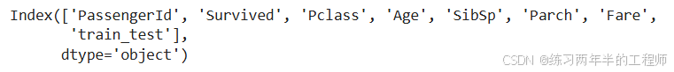
分离numeric data 和 categorical data

# quick way to separate numeric columns
training.describe().columns

输出：

training.columns

输出：

# look at numeric and categorical values separately
df_num = training[['Age', 'SibSp', 'Parch', 'Fare']]
df_cat = training[['Survived', 'Pclass', 'Sex', 'Ticket', 'Cabin', 'Embarked']]

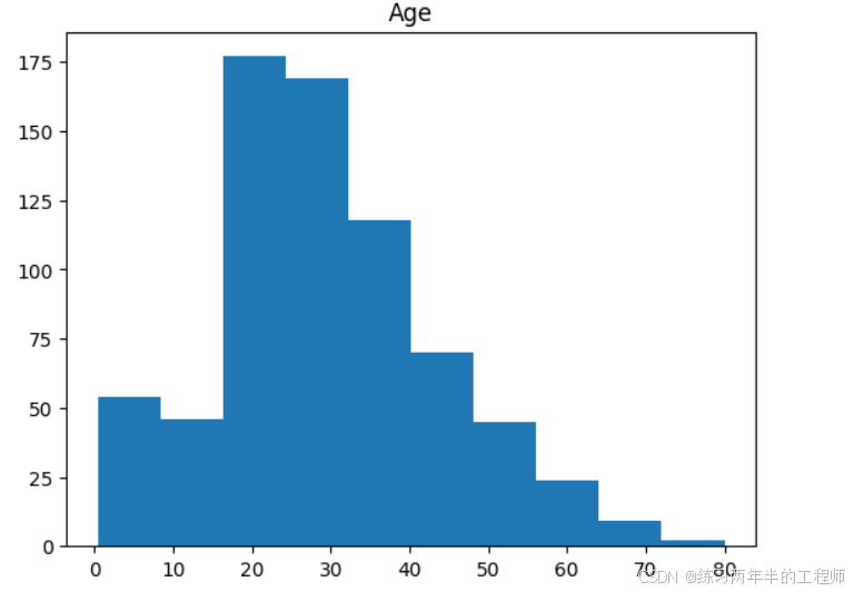
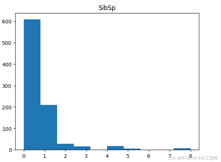
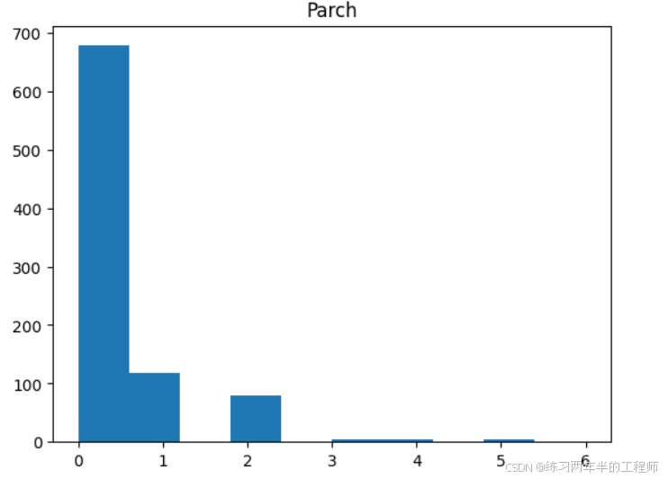
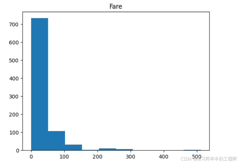
查看numeric data 的分布

#distribution for all numeric variables
for i in df_num.columns:
    plt.hist(df_num[i])
    plt.title(i)
    plt.show()

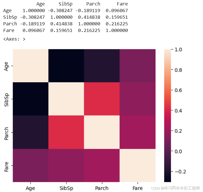
计算数据框中每两列之间的相关系数，绘制热力图，以矩阵形式展示数据框中列之间的相关性关系

print(df_num.corr())
sns.heatmap(df_num.corr())

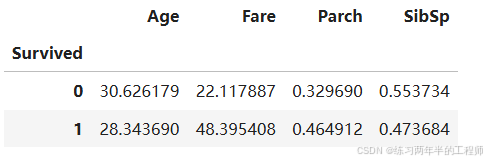
通过 Pandas 数据透视表 来比较不同变量（Age, SibSp, Parch, Fare）与目标变量（Survived）的关系

# compare survival rate across Age, SibSp, Parch, and Fare
pd.pivot_table(training, index='Survived', values=['Age', 'SibSp', 'Parch', 'Fare'])

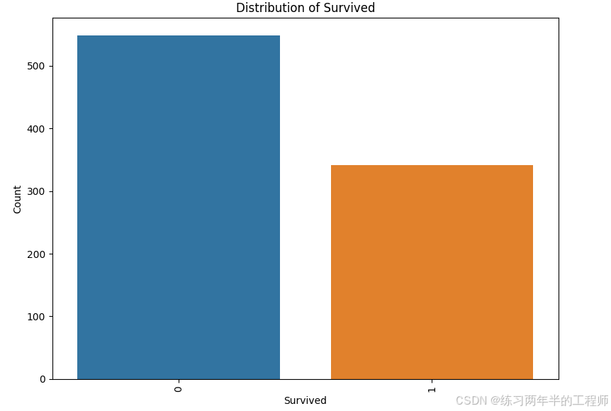
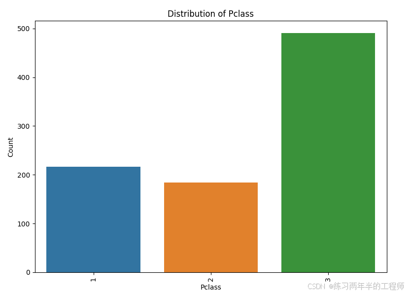
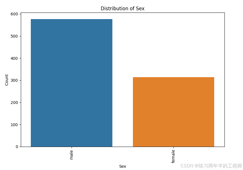
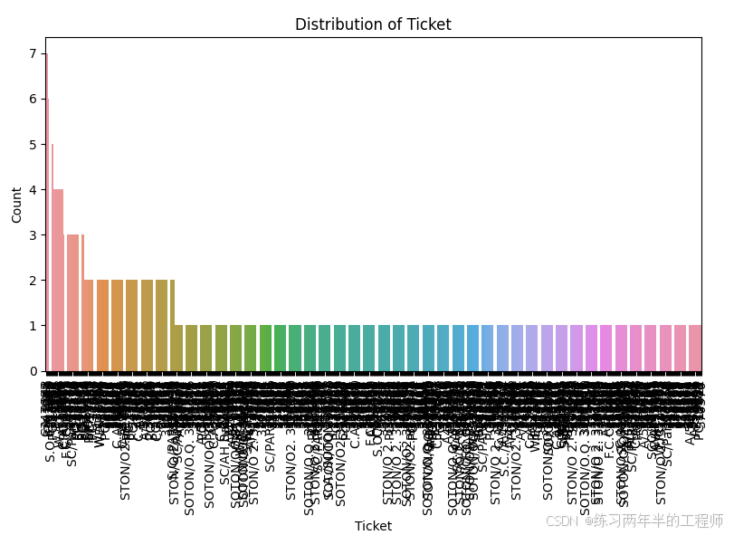
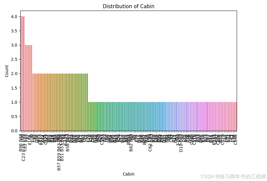
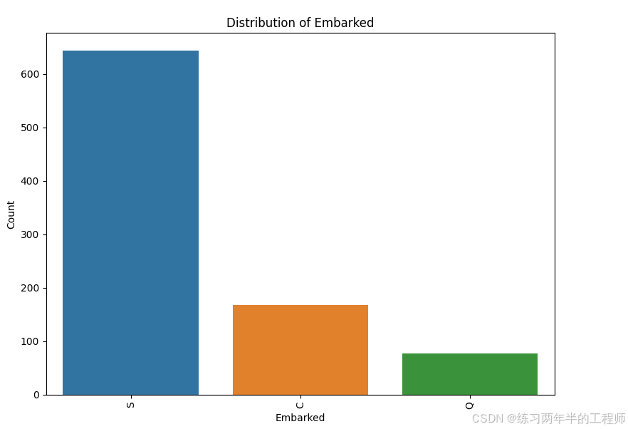
观察categorical data 的分布

for i in df_cat.columns:
    plt.figure(figsize=(8, 6))  # 设置图像大小
    value_counts = df_cat[i].value_counts()
    sns.barplot(x=value_counts.index, y=value_counts.values)
    plt.title(f'Distribution of {i}')
    plt.xlabel(i)
    plt.ylabel('Count')
    plt.xticks(rotation=90)  # 如果类别多，旋转标签避免重叠
    plt.tight_layout()       # 自动调整布局
    plt.show()

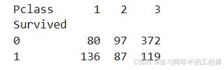
比较 Survived（是否生还） 和 Pclass（乘客舱位等级） 之间的关系

# Comparing survival and each of these categorical variables
print(pd.pivot_table(training, index = 'Survived', 
                     columns = 'Pclass',
                    values = 'Ticket',
                    aggfunc = 'count'))

假设 Ticket 是唯一标识乘客的字段，统计它的数量代表每组的乘客人数。

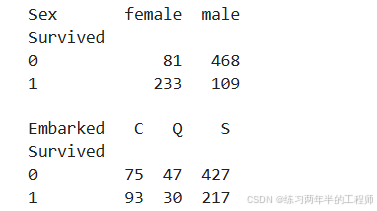
比较是否生还和性别、出发地之间的关系

print(pd.pivot_table(training, index = 'Survived', 
                     columns = 'Sex',
                    values = 'Ticket',
                    aggfunc = 'count'))
print()
print(pd.pivot_table(training, index = 'Survived', 
                     columns = 'Embarked',
                    values = 'Ticket',
                    aggfunc = 'count'))

Feature Engineering

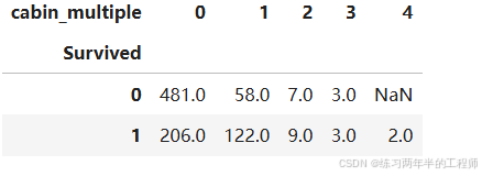
统计每位乘客的Cabin数量

training['cabin_multiple'] = training.Cabin.apply(
    lambda x: 0 if pd.isna(x) else len(x.split(' ')))

training['cabin_multiple'].value_counts()

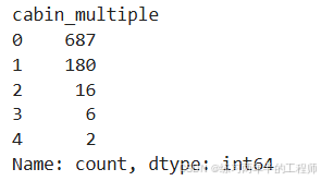
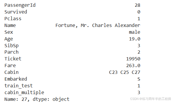
乘客可以有多个Cabin

training.iloc[27]

比较是否生还和Cabin数量的关系

pd.pivot_table(training, index = 'Survived', 
               columns = 'cabin_multiple', 
               values = 'Ticket',
              aggfunc = 'count')

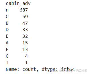
提取Cabin的首字母作单独的一列特征

# create categories based on the cabin letter (n stands for null)
# in this case, we will treat null values like it is own category

training['cabin_adv'] = training.Cabin.apply(
    lambda x: str(x)[0])

print(training.cabin_adv.value_counts())

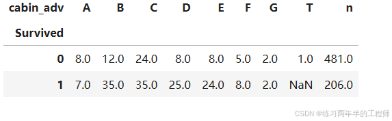
比较是否生还和Cabin首字母之间的关系

pd.pivot_table(training, index='Survived', 
               columns='cabin_adv',
              values='Name',
              aggfunc='count')

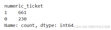
将Ticket分为单纯数字的和混杂的，提取Ticket中的字母部分

# understand ticket values better
# numeric vs non numeric

training['numeric_ticket'] = training.Ticket.apply(
    lambda x : 1 if x.isnumeric() else 0
)

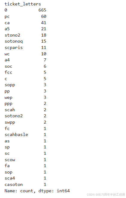
training['ticket_letters'] = training.Ticket.apply(
    lambda x: ''.join(x.split(' ')[:-1]).replace('.','').replace('/', '').lower() 
    if len(x.split(' ')[:-1]) > 0 else 0
)

training['numeric_ticket'].value_counts()

# view all rows in dataframe through scrolling

pd.set_option("display.max_rows", None)
training['ticket_letters'].value_counts()

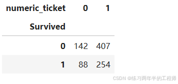
比较是否生还和Ticket数字的关系

# difference in numeric vs non-numeric tickets in survival rate
pd.pivot_table(training, index='Survived', 
               columns='numeric_ticket',
              values='Ticket',
              aggfunc='count')

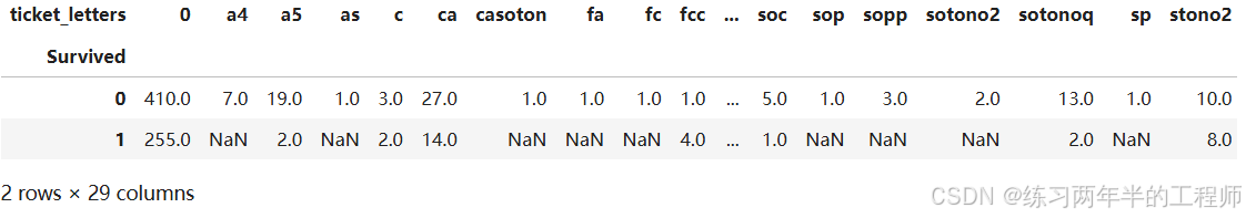
比较是否生还和Ticket字母的关系

# survival rate across different ticket types
pd.pivot_table(training, index='Survived', 
               columns='ticket_letters',
              values='Ticket',
              aggfunc='count')

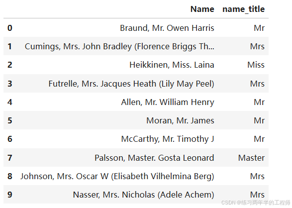
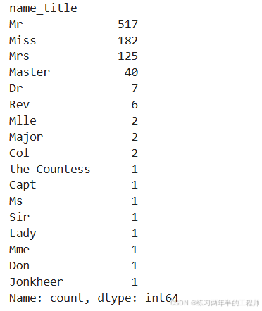
比较是否生还和名字title的关系

training['name_title'] = training.Name.apply(
    lambda x: x.split(',')[1].split('.')[0].strip()
)

training[["Name", "name_title"]].head(10)

training['name_title'].value_counts()

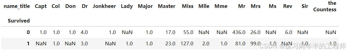
# survival rate across different name title
pd.pivot_table(training, index='Survived', 
               columns='name_title',
              values='Ticket',
              aggfunc='count')

Data Preprocessing

针对train和test的整体数据，重复以上的特征提取步骤，针对Cabin数量、Cabin首字母、Ticket的数字、Ticket的字母、名字的title

# create all categorical variables like the above for both training and testing
all_data['cabin_multiple'] = all_data.Cabin.apply(
    lambda x: 0 if pd.isna(x) else len(x.split(' ')))

all_data['cabin_adv'] = all_data.Cabin.apply(
    lambda x: str(x)[0])

all_data['numeric_ticket'] = all_data.Ticket.apply(
    lambda x : 1 if x.isnumeric() else 0
)

all_data['ticket_letters'] = all_data.Ticket.apply(
    lambda x: ''.join(x.split(' ')[:-1]).replace('.','').replace('/', '').lower() 
    if len(x.split(' ')[:-1]) > 0 else 0
)

all_data['name_title'] = all_data.Name.apply(
    lambda x: x.split(',')[1].split('.')[0].strip()
)

填补Age和Fare中的空白部分

# impute nulls for continuous data
all_data.Age = all_data.Age.fillna(training.Age.median())

all_data.Fare = all_data.Fare.fillna(training.Fare.median())

删除Embarked为空的行

# drop null 'embarked' rows. Only 2 instances of this in training and 0 in test
all_data.dropna(subset=['Embarked'], inplace = True)

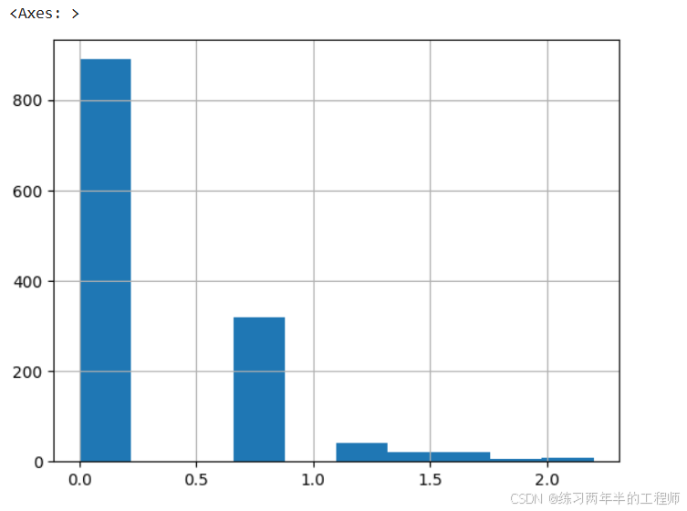
对 SibSp（兄弟姐妹/配偶数量）列进行 对数变换（log transformation），然后绘制 直方图 来查看变换后的数据分布

# tried log norm of sibsp 
all_data['norm_sibsp'] = np.log(all_data.SibSp + 1)
all_data['norm_sibsp'].hist()

进行对数变换，以减少数据的偏态（skewness），让分布更接近正态分布。
加 1 确保即使 SibSp = 0（没有兄弟姐妹或配偶），也不会报错（因为 log(0) 不定义）。

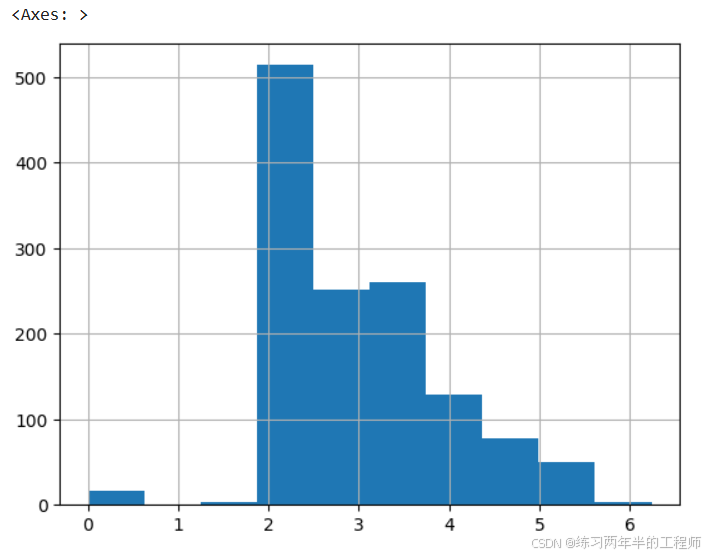
对Fare也进行对数变换

# log norm of fare
# normalized fare using logarithm to give more semblance of a normal distribution
all_data['norm_fare'] = np.log(all_data.Fare + 1)
all_data['norm_fare'].hist()

把Pclass改为string类型

all_data.Pclass = all_data.Pclass.astype(str)

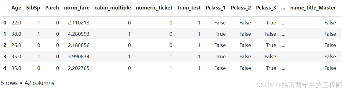
将分类数据转换为哑变量（即二进制变量），每个类别被转换成一个单独的列，列的值为 0 或 1，表示是否属于该类别

# create dummy variables from categories (also can use OneHotEncoder)

all_dummies = pd.get_dummies(all_data[[
    'Pclass',
    'Sex', 
    'Age', 
    'SibSp',
    'Parch',
    'norm_fare',
    'Embarked',
    'cabin_adv',
    'cabin_multiple',
    'numeric_ticket',
    'name_title',
    'train_test'
]])

机器学习算法（尤其是基于数学计算的算法，如线性回归和逻辑回归）通常无法直接处理非数值型数据。
哑变量将分类数据编码为数值型，同时保留了类别信息。

all_dummies.head()

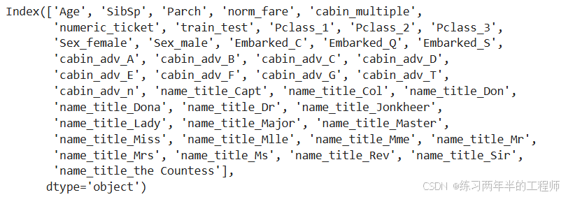
all_dummies.columns

再次分成train和test两种数据

# split to train test again

X_train = all_dummies[all_dummies.train_test == 1].drop(['train_test'], axis = 1)
X_test = all_dummies[all_dummies.train_test == 0].drop(['train_test'], axis = 1)

提取y_train作训练用的label

y_train = all_data[all_data.train_test == 1].Survived
y_train.shape

(889,)

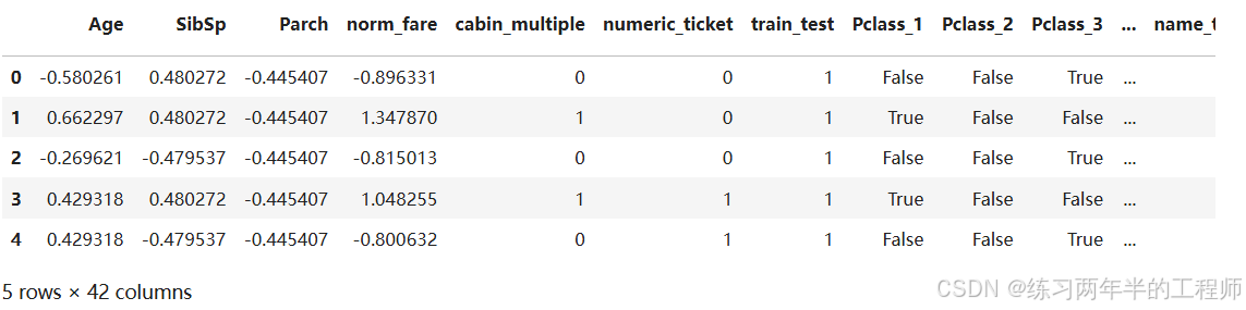
对某些连续型变量（Age, SibSp, Parch, norm_fare）进行标准化（standardization），即将其转换为均值为 0、标准差为 1 的分布

from sklearn.preprocessing import StandardScaler

scale = StandardScaler()
all_dummies_scaled = all_dummies.copy()
all_dummies_scaled[['Age', 'SibSp', 'Parch', 'norm_fare']] = scale.fit_transform(all_dummies_scaled[['Age', 'SibSp', 'Parch', 'norm_fare']])
all_dummies_scaled.head()

在机器学习模型（如逻辑回归、SVM、KNN 等）中，标准化可加快收敛速度，改善模型性能。

分开train和test的数据

X_train_scaled = all_dummies_scaled[all_dummies_scaled.train_test == 1].drop(['train_test'], axis=1)
X_test_scaled = all_dummies_scaled[all_dummies_scaled.train_test == 0].drop(['train_test'], axis=1)

y_train = all_data[all_data.train_test == 1].Survived

导入模型训练的packages

from sklearn.model_selection import cross_val_score
from sklearn.naive_bayes import GaussianNB
from sklearn.linear_model import LogisticRegression
from sklearn import tree
from sklearn.neighbors import KNeighborsClassifier
from sklearn.ensemble import RandomForestClassifier
from sklearn.svm import SVC

使用 朴素贝叶斯分类器 (Naive Bayes) 作为基准模型（baseline）来完成分类任务，并通过交叉验证评估模型性能

# usually use Naive Bayes as a baseline for classification tasks

gnb = GaussianNB()
cv = cross_val_score(gnb, X_train_scaled, y_train, cv = 5)
print(cv)
print(cv.mean())

将数据分为 5 份，进行 5 折交叉验证，每次用 4 份训练、1 份验证。
输出：

[0.66853933 0.70224719 0.75842697 0.74719101 0.73446328]
0.7221735542436362

使用 逻辑回归模型 (Logistic Regression) 来完成分类任务，并通过交叉验证评估其性能

lr = LogisticRegression(max_iter = 2000)
lr_cv = cross_val_score(lr, X_train, y_train, cv = 5)
print(lr_cv)
print(lr_cv.mean())

逻辑回归使用迭代优化算法（如梯度下降）来求解。
该参数设置最大迭代次数为 2000（默认值为 100），确保模型可以收敛，即找到最佳参数。
输出：

[0.8258427  0.80898876 0.80337079 0.82022472 0.85310734]
0.8223068621849807

lr = LogisticRegression(max_iter = 2000)
lr_cv_scaled = cross_val_score(lr, X_train_scaled, y_train, cv = 5)
print(lr_cv_scaled)
print(lr_cv_scaled.mean())

输出：

[0.8258427  0.80898876 0.80337079 0.82022472 0.85310734]
0.8223068621849807

使用 决策树分类器 (DecisionTreeClassifier) 来完成分类任务，并通过交叉验证评估其性能

dt = tree.DecisionTreeClassifier(random_state = 1)
dt_cv = cross_val_score(dt, X_train, y_train, cv = 5)
print(dt_cv)
print(dt_cv.mean())

[0.75842697 0.74719101 0.8258427  0.74719101 0.8079096 ]
0.7773122579826065

dt_new = tree.DecisionTreeClassifier(random_state = 1)
dt_cv_scaled = cross_val_score(dt_new, X_train_scaled, y_train, cv = 5)
print(dt_cv_scaled)
print(dt_cv_scaled.mean())

[0.75842697 0.74719101 0.8258427  0.74719101 0.8079096 ]
0.7773122579826065

使用 K 近邻分类器 (K-Nearest Neighbors, KNN) 来完成分类任务，并通过交叉验证评估其性能

knn = KNeighborsClassifier()
knn_cv = cross_val_score(knn, X_train, y_train, cv = 5)
print(knn_cv)
print(knn_cv.mean())

输出：

[0.76966292 0.79775281 0.80898876 0.82022472 0.85310734]
0.8099473116231829

knn = KNeighborsClassifier()
knn_cv_scaled = cross_val_score(knn, X_train_scaled, y_train, cv = 5)
print(knn_cv_scaled)
print(knn_cv_scaled.mean())

输出：

[0.79775281 0.79213483 0.83146067 0.79775281 0.85310734]
0.8144416936456548

KNN 是一种基于距离的非参数分类算法，通过寻找样本的 K 个最近邻居 来决定分类标签。
KNN 的性能受数据特征尺度和距离度量方式的影响。建议在使用前对特征进行标准化（如用 StandardScaler）。
KNN 的时间复杂度较高，尤其在大数据集和高维数据中，因为需要计算所有点之间的距离。

使用 随机森林分类器 (Random Forest Classifier) 完成分类任务，并通过交叉验证评估其性能

rf = RandomForestClassifier(random_state = 1)
rf_cv = cross_val_score(rf, X_train, y_train, cv = 5)
print(rf_cv)
print(rf_cv.mean())

[0.80898876 0.79213483 0.84831461 0.73595506 0.82485876]
0.8020504030978227

rf = RandomForestClassifier(random_state = 1)
rf_cv = cross_val_score(rf, X_train_scaled, y_train, cv = 5)
print(rf_cv)
print(rf_cv.mean())

[0.80337079 0.79213483 0.84831461 0.73595506 0.82485876]
0.8009268075922046

• 随机森林通过构建多个决策树，并对它们的预测结果进行投票或平均来完成分类任务。
• 集成方法：每棵树是从训练数据的随机子集生成的。
• 减少过拟合：通过随机性和多个树的投票机制。
• 随机森林能够有效应对高维数据和多样性特征。

使用 支持向量机分类器 (Support Vector Classifier, SVC) 完成分类任务，并通过交叉验证评估其性能

svc = SVC(probability = True)
svc_cv = cross_val_score(svc, X_train_scaled, y_train, cv=5)
print(svc_cv)
print(svc_cv.mean())

[0.85393258 0.82022472 0.8258427  0.80337079 0.86440678]
0.8335555132355742

SVM 对高维数据非常有效，适合处理复杂的非线性问题。
SVM 对特征尺度非常敏感，必须对输入特征进行标准化或归一化（如使用 StandardScaler）。
对于大型数据集，训练时间可能较长，因为 SVM 的时间复杂度与样本数量的平方成正比。

使用 XGBoost 分类器 (XGBClassifier) 进行分类任务，并通过交叉验证评估其性能

from xgboost import XGBClassifier
xgb = XGBClassifier(random_state = 1)
xgb_cv = cross_val_score(xgb, X_train_scaled, y_train, cv = 5)
print(xgb_cv)
print(xgb_cv.mean())

[0.80337079 0.80898876 0.85393258 0.78651685 0.80225989]
0.8110137751539389

一种基于决策树的提升 (boosting) 方法，特别适合处理大规模数据集的分类和回归问题。
提供了高效的实现和丰富的参数设置，在许多机器学习竞赛中表现出色。
与随机森林相比，XGBoost 通常能提供更高的准确率，但训练时间可能更长。

使用 投票分类器 (VotingClassifier) 对多个模型进行集成，通过交叉验证评估其性能

from sklearn.ensemble import VotingClassifier
voting_clf = VotingClassifier(estimators = 
                             [('lr', lr),
                             ('knn', knn),
                             ('rf', rf),
                             ('gnb', gnb),
                             ('svc', svc),
                             ('xgb', xgb)], voting = 'soft')
voting_cv = cross_val_score(voting_clf, X_train_scaled, y_train, cv = 5)
print(voting_cv)
print(voting_cv.mean())

[0.83146067 0.81460674 0.83146067 0.79775281 0.84745763]
0.8245477051990097

结合多个模型的预测结果来提高分类任务的性能。
voting=‘hard’：根据多数票决策（模型预测标签的频率）。
voting=‘soft’：根据预测概率的平均值进行决策（权重可调）。

训练投票分类器，用测试数据预测目标变量，将预测结果格式化为所需的提交文件

voting_clf.fit(X_train_scaled, y_train)
y_hat_base_vc = voting_clf.predict(X_test_scaled).astype(int)
basic_submission = {'PassengerId': test.PassengerId, 'Survived': y_hat_base_vc}
base_submission = pd.DataFrame(data = basic_submission)
base_submission.to_csv('base_submission.csv', index=False)

调整模型

导入调整模型所需的packages

from sklearn.model_selection import GridSearchCV
from sklearn.model_selection import RandomizedSearchCV

准备一个function用来打印最佳的结果和参数

# performance reporting function

def clf_performance(classifier, model_name):
    print(model_name)
    print('Best Score: ' + str(classifier.best_score_))
    print('Best Parameters: ' + str(classifier.best_params_))

通过网格搜索 (GridSearchCV) 对逻辑回归模型 (LogisticRegression) 的超参数进行优化，找到性能最优的参数组合，并评估模型的性能

lr = LogisticRegression()
param_grid = {'max_iter': [2000],
             'penalty': ['l1', 'l2'],
             'C': np.logspace(-4, 4, 20),
             'solver': ['liblinear']}

clf_lr = GridSearchCV(lr, param_grid = param_grid, cv = 5,
                     verbose = True, n_jobs = -1)
best_clf_lr = clf_lr.fit(X_train_scaled, y_train)
clf_performance(best_clf_lr, 'Logistic Regression')

verbose = True：输出搜索进度的详细信息。
n_jobs = -1：并行计算，使用所有可用的 CPU 核心。

输出：

Fitting 5 folds for each of 40 candidates, totalling 200 fits
Logistic Regression
Best Score: 0.8279375357074843
Best Parameters: {'C': 1.623776739188721, 'max_iter': 2000, 'penalty': 'l1', 'solver': 'liblinear'}

通过网格搜索 (GridSearchCV) 优化 K-近邻分类器 (KNeighborsClassifier) 的超参数，找到最佳配置以提高模型性能，并对结果进行评估

knn = KNeighborsClassifier()
param_grid = {'n_neighbors': [3,5,7,9],
             'weights': ['uniform', 'distance'],
             'algorithm': ['auto', 'ball_tree', 'kd_tree'],
             'p': [1,2]}

clf_knn = GridSearchCV(knn, param_grid = param_grid, cv = 5,
                      verbose = True, n_jobs = -1)
best_clf_knn = clf_knn.fit(X_train_scaled, y_train)
clf_performance(best_clf_knn, 'KNN')

‘uniform’：所有邻居的权重相同。
‘distance’：邻居权重与距离成反比，较近的邻居影响更大。
p=1：曼哈顿距离。
p=2：欧几里得距离。

输出：

Fitting 5 folds for each of 48 candidates, totalling 240 fits
KNN
Best Score: 0.8290611312131023
Best Parameters: {'algorithm': 'ball_tree', 'n_neighbors': 7, 'p': 2, 'weights': 'uniform'}

使用网格搜索 (GridSearchCV) 优化支持向量机分类器 (SVC) 的超参数，以找到最佳配置，并评估其性能

svc = SVC(probability = True)
param_grid = tuned_parameters = [{'kernel': ['rbf'], 
'gamma': [.1, .5, 1, 2, 5, 10], 'C': [.1, 1, 10, 100, 1000]},
{'kernel': ['linear'],'C': [.1, 1, 10, 100, 1000]},
{'kernel': ['poly'], 'degree': [2,3,4,5], 'C': [.1, 1, 10, 100, 1000]}]

clf_svc = GridSearchCV(svc, param_grid = param_grid, 
                       cv = 5, verbose = True, n_jobs = -1)
best_clf_svc = clf_svc.fit(X_train_scaled, y_train)
clf_performance(best_clf_svc, 'SVC')

rbf（径向基函数）内核：该内核函数使用 gamma 和 C 作为超参数。
gamma 控制高维空间中数据点的影响范围。较小的值表示较远的点有影响，较大的值则表示较近的点主导。
C 控制正则化强度，较大的值意味着模型对错误分类点的惩罚较大。

输出：

Fitting 5 folds for each of 55 candidates, totalling 275 fits
SVC
Best Score: 0.8335555132355742
Best Parameters: {'C': 1, 'gamma': 0.1, 'kernel': 'rbf'}

使用网格搜索优化 随机森林分类器（Random Forest Classifier）超参数，并评估优化后的模型性能

rf = RandomForestClassifier(random_state = 1)
param_grid = {'n_estimators': [400, 450, 500, 550],
             'criterion': ['gini', 'entropy'],
             'bootstrap': [True],
             'max_depth': [15, 20, 25],
             'max_features': ['auto', 'sqrt', 10],
             'min_samples_leaf': [2, 3],
             'min_samples_split': [2, 3]}
clf_rf = GridSearchCV(rf, param_grid = param_grid, cv = 5,
                     verbose = True, n_jobs = -1)
best_clf_rf = clf_rf.fit(X_train_scaled, y_train)
clf_performance(best_clf_rf, 'Random Forest')

• n_estimators：森林中树木的数量。
• criterion：用于分裂节点的标准，选择 gini 或 entropy。这两者分别是 Gini 不纯度 和 信息增益，常用于衡量每个分裂的质量。
• bootstrap：是否使用自助法（Bootstrapping）进行训练，选择 True 代表使用自助采样（即从训练数据中有放回地采样）。
• max_depth：树的最大深度，防止模型过拟合。
• max_features：决定每棵树使用多少特征进行训练。选择 auto、sqrt 或一个固定值（如 10）。auto 表示使用所有特征，sqrt 表示使用特征总数的平方根。
• min_samples_leaf：每个叶节点的最小样本数。值越大，树越简单，减少过拟合的风险。
• min_samples_split：分裂一个节点所需的最小样本数。通过调整这个值，可以控制树的生长过程，避免过度分裂。

输出：

Fitting 5 folds for each of 288 candidates, totalling 1440 fits
Random Forest
Best Score: 0.8358027042468101
Best Parameters: {'bootstrap': True, 'criterion': 'gini', 'max_depth': 15, 'max_features': 10, 'min_samples_leaf': 3, 'min_samples_split': 2, 'n_estimators': 550}

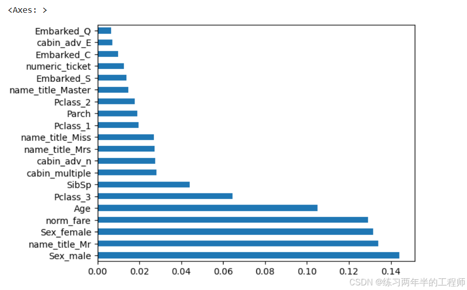
绘制出前20个最重要特征的水平条形图

best_rf = best_clf_rf.best_estimator_.fit(X_train_scaled, y_train)
feat_importances = pd.Series(best_rf.feature_importances_, 
                             index = X_train_scaled.columns)
feat_importances.nlargest(20).plot(kind = 'barh')

• best_clf_rf.best_estimator_：这个属性返回的是最优随机森林模型（经过调优后的），即该模型在进行网格搜索时表现最好的模型。
• best_rf.feature_importances_：这是一个 RandomForestClassifier 模型的属性，表示每个特征的重要性。该属性是一个数组，数组的每个元素对应于训练数据集中每个特征的“重要性”分数。重要性分数越高，意味着该特征对模型预测的影响越大。
• feat_importances.nlargest(20)：nlargest(20) 会从 feat_importances 中选择出 重要性最高的20个特征。这个方法返回前20个重要性分数最大的特征（如果特征总数超过20个）。这个步骤用于筛选最具代表性的特征，而不是显示所有特征。
• plot 方法用于绘制数据的图形。在这里，使用 kind=‘barh’ 来绘制水平条形图（barh = bar horizontal）。

输出：

使用了XGBoost（极梯度提升树）分类器，并通过GridSearchCV来优化模型超参数，最终选择最优模型并评估其表现

xgb = XGBClassifier(random_state = 1)

param_grid = {
    'n_estimators': [450, 500, 550],
    'colsample_bytree': [0.75, 0.8, 0.85],
    'max_depth': [None],
    'reg_alpha': [1],
    'reg_lambda': [2, 5, 10],
    'subsample': [0.55, 0.6, 0.65],
    'learning_rate': [0.5],
    'gamma': [.5, 1, 2],
    'min_child_weight': [0.01],
    'sampling_method': ['uniform']
}

clf_xgb = GridSearchCV(xgb, param_grid = param_grid, 
                      cv = 5, verbose = True, n_jobs = -1)
best_clf_xgb = clf_xgb.fit(X_train_scaled, y_train)
clf_performance(best_clf_xgb, 'XGB')

• colsample_bytree: [0.75, 0.8, 0.85]：这个参数控制每棵树的训练数据特征的采样比例。值越小，模型的多样性越大，但可能损失一些准确性。
• max_depth: [None]：max_depth 参数控制树的最大深度。深度越大，树就越复杂，容易过拟合；None 表示不限制深度。
• reg_alpha: [1]：reg_alpha 是 L1 正则化参数。它控制正则化的强度，越大则对模型的约束越强，防止过拟合。
• reg_lambda: [2, 5, 10]：reg_lambda 是 L2 正则化参数。与 L1 正则化类似，它控制正则化强度，防止过拟合。
• subsample: [0.55, 0.6, 0.65]：这个参数控制每棵树训练时使用的样本比例。值越小，模型的多样性越大，可能提高泛化能力，但也可能降低准确性。
• gamma: [0.5, 1, 2]：gamma 是节点分裂所需的最小损失减少量。较大的 gamma 会使得树的结构更加简单，从而减少过拟合。

输出：

Fitting 5 folds for each of 243 candidates, totalling 1215 fits
XGB
Best Score: 0.8504030978226369
Best Parameters: {'colsample_bytree': 0.75, 'gamma': 0.5, 'learning_rate': 0.5, 'max_depth': None, 'min_child_weight': 0.01, 'n_estimators': 550, 'reg_alpha': 1, 'reg_lambda': 10, 'sampling_method': 'uniform', 'subsample': 0.65}

用测试数据预测目标变量，将预测结果格式化为所需的提交文件

y_hat_xgb = best_clf_xgb.best_estimator_.predict(X_test_scaled).astype(int)
xgb_submission = {'PassengerId': test.PassengerId, 'Survived': y_hat_xgb}
submission_xgb = pd.DataFrame(data = xgb_submission)
submission_xgb.to_csv('xgb_submission.csv', index=False)

将Grid Search得到的最优模型放入Voting Classifier

best_lr = best_clf_lr.best_estimator_
best_knn = best_clf_knn.best_estimator_
best_svc = best_clf_svc.best_estimator_
best_rf = best_clf_rf.best_estimator_
best_xgb = best_clf_xgb.best_estimator_

voting_clf_hard = VotingClassifier(
    estimators = [('knn', best_knn),
                 ('rf', best_rf),
                 ('svc', best_svc)], voting = 'hard'
)

voting_clf_soft = VotingClassifier(
    estimators = [('knn', best_knn),
                 ('rf', best_rf),
                 ('svc', best_svc)], voting = 'soft'
)

voting_clf_all = VotingClassifier(
    estimators = [('knn', best_knn),
                 ('rf', best_rf),
                 ('svc', best_svc),
                 ('lr', best_lr)], voting = 'soft'
)

voting_clf_xgb = VotingClassifier(
    estimators = [('knn', best_knn),
                 ('rf', best_rf),
                 ('svc', best_svc),
                 ('xgb', best_xgb)], voting = 'soft'
)

knn, rf, svc - hard voting classifier

vc_hard_res = cross_val_score(voting_clf_hard, X_train, y_train, cv = 5)
print('voting_clf_hard: ', vc_hard_res)
print('voting_clf_hard mean: ', vc_hard_res.mean())

输出：

voting_clf_hard:  [0.79213483 0.81460674 0.82022472 0.79775281 0.83615819]
voting_clf_hard mean:  0.8121754586427983

knn, rf, svc - soft voting classifier

vc_soft_res = cross_val_score(voting_clf_soft, X_train, y_train, cv = 5)
print('voting_clf_soft: ', vc_soft_res)
print('voting_clf_soft mean: ', vc_soft_res.mean())

输出：

voting_clf_soft:  [0.78651685 0.8258427  0.81460674 0.79775281 0.85310734]
voting_clf_soft mean:  0.8155652891512728

knn, rf, svc, lr - soft voting classifier

vc_all_res = cross_val_score(voting_clf_all, X_train, y_train, cv = 5)
print('voting_clf_all: ', vc_all_res)
print('voting_clf_all mean: ', vc_all_res.mean())

输出：

voting_clf_all:  [0.80898876 0.83146067 0.8258427  0.80898876 0.85875706]
voting_clf_all mean:  0.8268075922046595

knn, rf, svc, xgb - soft voting classifier

vc_xgb_res = cross_val_score(voting_clf_xgb, X_train, y_train, cv = 5)
print('voting_clf_xgb: ', vc_xgb_res)
print('voting_clf_xgb mean: ', vc_xgb_res.mean())

输出：

voting_clf_xgb:  [0.83146067 0.82022472 0.84269663 0.80898876 0.85310734]
voting_clf_xgb mean:  0.8312956262299244

探索在soft voting classifier中，weight对于model的影响

# in a soft voting classifier, you can weight some models more
# than others. Use a grid search to explore different weightings

params = {'weights': [[1,1,1], [1,2,1], [1,1,2], [2,1,1], [2,2,1],
                     [1,2,2], [2,1,2]]}

vote_weight = GridSearchCV(voting_clf_soft, param_grid = params,
                          cv = 5, verbose = True, n_jobs = -1)
best_clf_weight = vote_weight.fit(X_train_scaled, y_train)
clf_performance(best_clf_weight, 'VC Weights')

输出：

Fitting 5 folds for each of 7 candidates, totalling 35 fits
VC Weights
Best Score: 0.83244461372437
Best Parameters: {'weights': [2, 2, 1]}

进行预测

voting_clf_hard.fit(X_train_scaled, y_train)
voting_clf_soft.fit(X_train_scaled, y_train)
voting_clf_all.fit(X_train_scaled, y_train)
voting_clf_xgb.fit(X_train_scaled, y_train)
best_rf.fit(X_train_scaled, y_train)

y_hat_vc_hard = voting_clf_hard.predict(X_test_scaled).astype(int)
y_hat_rf = best_rf.predict(X_test_scaled).astype(int)
y_hat_vc_soft = voting_clf_soft.predict(X_test_scaled).astype(int)
y_hat_vc_all = voting_clf_all.predict(X_test_scaled).astype(int)
y_hat_vc_xgb = voting_clf_xgb.predict(X_test_scaled).astype(int)

rf_data = {'PassengerId': test.PassengerId, 'Survived': y_hat_rf}
rf_submission = pd.DataFrame(data = rf_data)

vc_hard_data = {'PassengerId': test.PassengerId, 'Survived': y_hat_vc_hard}
vc_hard_submission = pd.DataFrame(data = vc_hard_data)

vc_soft_data = {'PassengerId': test.PassengerId, 'Survived': y_hat_vc_soft}
vc_soft_submission = pd.DataFrame(data = vc_soft_data)

vc_all_data = {'PassengerId': test.PassengerId, 'Survived': y_hat_vc_all}
vc_all_submission = pd.DataFrame(data = vc_all_data)

vc_xgb_data = {'PassengerId': test.PassengerId, 'Survived': y_hat_vc_xgb}
vc_xgb_submission = pd.DataFrame(data = vc_xgb_data)

final_data_comp = {'PassengerId': test.PassengerId,
                  'Survived_vc_hard': y_hat_vc_hard,
                  'Survived_rf': y_hat_rf,
                  'Survived_vc_soft': y_hat_vc_soft,
                  'Survived_vc_all': y_hat_vc_all,
                  'Survived_vc_xgb': y_hat_vc_xgb}

comparison = pd.DataFrame(data = final_data_comp)

比较不同模型的差异

# track differences between outputs
comparison['difference_rf_vc_hard'] = comparison.apply(
    lambda x: 1 if x.Survived_vc_hard != x.Survived_rf else 0,
    axis = 1
)

comparison['difference_soft_hard'] = comparison.apply(
    lambda x: 1 if x.Survived_vc_hard != x.Survived_vc_soft else 0,
    axis = 1
)

comparison['difference_hard_all'] = comparison.apply(
    lambda x: 1 if x.Survived_vc_all != x.Survived_vc_hard else 0,
    axis = 1
)

comparison.difference_hard_all.value_counts()

输出：

difference_hard_all
0    410
1      8
Name: count, dtype: int64

准备提交文件

#prepare submission files 
rf_submission.to_csv('submission_rf.csv', index =False)
vc_hard_submission.to_csv('submission_vc_hard.csv',index=False)
vc_soft_submission.to_csv('submission_vc_soft.csv', index=False)
vc_all_submission.to_csv('submission_vc_all.csv', index=False)
vc_xgb_submission.to_csv('submission_vc_xgb2.csv', index=False)