


跟着小土堆学习pytorch(三)
继续学习。
现有网络模型的使用及修改
本节内容主要跟着up主学习有关模型的使用和修改,以分类问题为主,模型使用VGG,数据集仍为 CIFAR10 数据集(主要用于分类)。
数据集 ImageNet
注意:必须要先有 package scipy
在 Terminal 里输入
pip list
寻找是否有 scipy,若没有的话输入
pip install scipy
但在教学中由于该数据集并未公开访问,需要别的路径下载(可以直接搜索ImageNet下载),并且由于该数据集过于庞大,因此课程并没有继续使用。
以下是下载该数据集的一些参数:
相关代码:
import torchvision

train_data = torchvision.datasets.ImageNet("./data_image_net", split='train', download=True, transform=torchvision.transforms.ToTensor)
这里并没有下载成功,而是报错了,原因上面讲过,并且课程后续并未使用。
VGG16 模型
VGG 11/13/16/19 常用16和19。
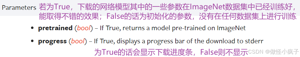
参数:Pretrained
import torchvision
from torch import nn
vgg16_false = torchvision.models.vgg16(pretrained=False)
vgg16_true = torchvision.models.vgg16(pretrained=True) # 需要进行下载
可以和up主一样打断点来查看相关的权重。
总结:
- 设置为 False 的情况,相当于网络模型中的参数都是初始化的、默认的
- 设置为 True 时,网络模型中的参数在数据集上是训练好的,能达到比较好的效果
接下来可以查看下vgg16的网络架构:print(vgg16_true ),如下所示:
VGG(
  (features): Sequential(
    (0): Conv2d(3, 64, kernel_size=(3, 3), stride=(1, 1), padding=(1, 1))
    (1): ReLU(inplace=True)
    (2): Conv2d(64, 64, kernel_size=(3, 3), stride=(1, 1), padding=(1, 1))
    (3): ReLU(inplace=True)
    (4): MaxPool2d(kernel_size=2, stride=2, padding=0, dilation=1, ceil_mode=False)
    (5): Conv2d(64, 128, kernel_size=(3, 3), stride=(1, 1), padding=(1, 1))
    (6): ReLU(inplace=True)
    (7): Conv2d(128, 128, kernel_size=(3, 3), stride=(1, 1), padding=(1, 1))
    (8): ReLU(inplace=True)
    (9): MaxPool2d(kernel_size=2, stride=2, padding=0, dilation=1, ceil_mode=False)
    (10): Conv2d(128, 256, kernel_size=(3, 3), stride=(1, 1), padding=(1, 1))
    (11): ReLU(inplace=True)
    (12): Conv2d(256, 256, kernel_size=(3, 3), stride=(1, 1), padding=(1, 1))
    (13): ReLU(inplace=True)
    (14): Conv2d(256, 256, kernel_size=(3, 3), stride=(1, 1), padding=(1, 1))
    (15): ReLU(inplace=True)
    (16): MaxPool2d(kernel_size=2, stride=2, padding=0, dilation=1, ceil_mode=False)
    (17): Conv2d(256, 512, kernel_size=(3, 3), stride=(1, 1), padding=(1, 1))
    (18): ReLU(inplace=True)
    (19): Conv2d(512, 512, kernel_size=(3, 3), stride=(1, 1), padding=(1, 1))
    (20): ReLU(inplace=True)
    (21): Conv2d(512, 512, kernel_size=(3, 3), stride=(1, 1), padding=(1, 1))
    (22): ReLU(inplace=True)
    (23): MaxPool2d(kernel_size=2, stride=2, padding=0, dilation=1, ceil_mode=False)
    (24): Conv2d(512, 512, kernel_size=(3, 3), stride=(1, 1), padding=(1, 1))
    (25): ReLU(inplace=True)
    (26): Conv2d(512, 512, kernel_size=(3, 3), stride=(1, 1), padding=(1, 1))
    (27): ReLU(inplace=True)
    (28): Conv2d(512, 512, kernel_size=(3, 3), stride=(1, 1), padding=(1, 1))
    (29): ReLU(inplace=True)
    (30): MaxPool2d(kernel_size=2, stride=2, padding=0, dilation=1, ceil_mode=False)
  )
  (avgpool): AdaptiveAvgPool2d(output_size=(7, 7))
  (classifier): Sequential(
    (0): Linear(in_features=25088, out_features=4096, bias=True)
    (1): ReLU(inplace=True)
    (2): Dropout(p=0.5, inplace=False)
    (3): Linear(in_features=4096, out_features=4096, bias=True)
    (4): ReLU(inplace=True)
    (5): Dropout(p=0.5, inplace=False)
    (6): Linear(in_features=4096, out_features=1000, bias=True)
  )
)
- 在其结构上进行添加层,可以选择不同的位置进行添加(总体结构或者classifier中):
# 在总体中添加
# vgg16_true.add_module("add_linear", module=nn.Linear(1000, 10))
# 在classifier中添加:
vgg16_true.classifier.add_module("add_linear", module=nn.Linear(1000, 10))
在网络最后添加:
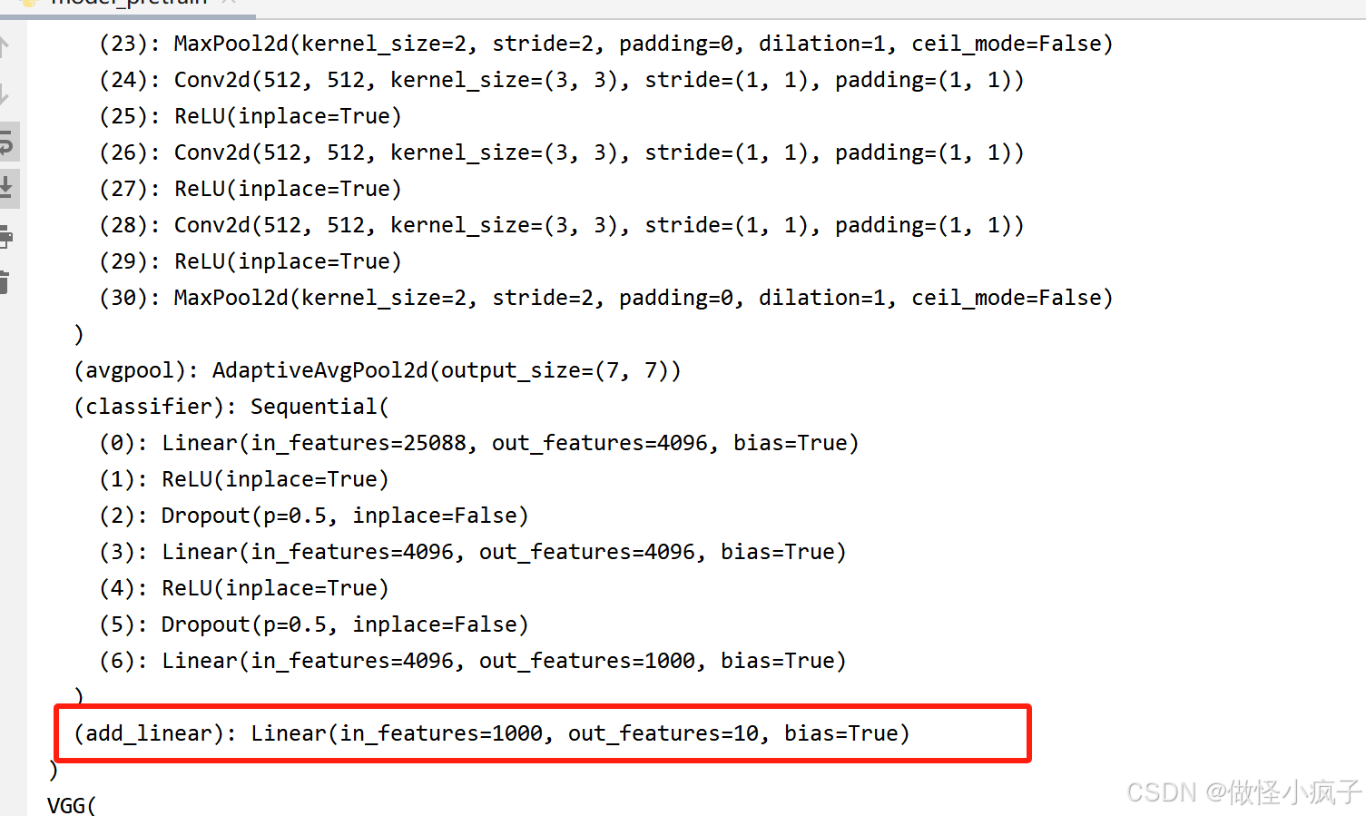
在classifier中添加:
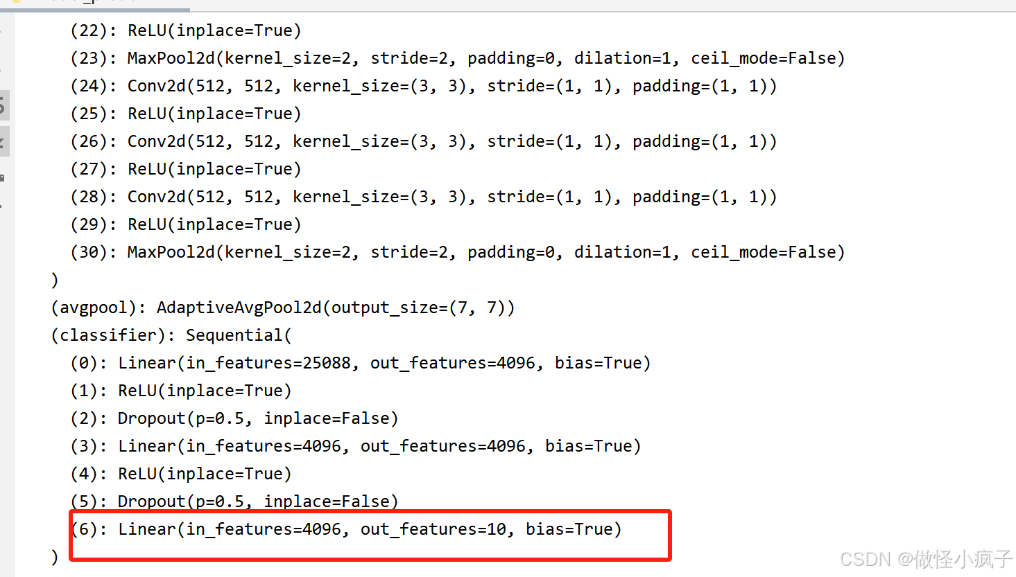
- 修改已有的网络
# 修改现有的网络:
vgg16_false.classifier[6] = nn.Linear(4096, 10)
print(vgg16_false)
结果如下: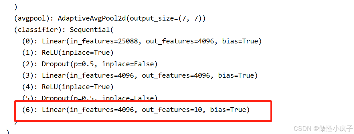
网络模型的保存与读取
网络模型的保存有两种方式
-
方法1:不仅保存了模型的结构,还保存了模型的参数
torch.save(vgg16, "vgg16_method1.pth") -
保存方式2: 模型参数(官方推荐): 保存为字典模式
torch.save(vgg16.state_dict(), "vgg16_method2.pth")
运行完代码之后就会有两个这样的文件:
模型的读取
- 模型保存方式1的读取方式:直接使用
torch.load("path")
vgg_model1 = torch.load("vgg16_method1.pth")
print(vgg_model1)
- 模型保存方式2的读取方式:
vgg_model2 = torch.load("vgg16_method2.pth")
print((vgg_model2))

# 将字典模式的参数加载到模型中:
# 先定义模型
vgg16 = torchvision.models.vgg16(pretrained=False)
# 使用load_state_dict 来加载
vgg16.load_state_dict(torch.load("vgg16_method2.pth"))
print(vgg16)
使用以上的方式就可以读取模型。
- 使用方式1可能出现的问题(陷阱)
如下代码所示,定义一个模型,然后,将该模型使用方式1进行保存
# 陷阱:
class Test(nn.Module):
    def __init__(self):
        super(Test, self).__init__()
        self.conv1 = nn.Conv2d(3, 64, kernel_size=3)

    def forward(self, x):
        output = self.conv1(x)
        return output

test = Test()

torch.save(test, "test_model1.pth")
在另一个文件夹进行读取文件的时候,可能会报错,代码如下:
## 陷阱
class Test(nn.Module):
    def __init__(self):
        super(Test, self).__init__()
        self.conv1 = nn.Conv2d(3, 64, kernel_size=3)

    def forward(self, x):
        output = self.conv1(x)
        return output
model = torch.load("test_model1.pth")
print(model)
# 报错: Can't get attribute 'Test' on <module '__main__' from 'D:/learning/pytorch/learn_pytorch/model_load.py'>
# 解决:需要将模型再写一遍 & 或者 将模型引入from model_save import * (真实项目中不会把模型移来移去)
完整的模型训练套路(CIFAR10数据集)
创建model.py,搭建神经网络模型
如下所示:
# 搭建神经网络
import torch
from torch import nn

class Test(nn.Module):

    def __init__(self) :
        super(Test, self).__init__()
        self.model = nn.Sequential(
            nn.Conv2d(3, 32, 5, 1, 2),
            nn.MaxPool2d(2),
            nn.Conv2d(32, 32, 5, 1, 2),
            nn.MaxPool2d(2),
            nn.Conv2d(32, 64, 5, 1, 2),
            nn.MaxPool2d(2),
            nn.Flatten(),
            nn.Linear(64 * 4 * 4, 64),
            nn.Linear(64, 10)
        )

    def forward(self, x):
        x = self.model(x)
        return x

# main函数
if __name__ == '__main__':
    test = Test()
    # 验证网络模型的正确性,创造一个输入尺寸,判断输出尺寸是不是我们想要的
    input = torch.ones((64, 3, 32, 32))  # batchsize=64,channel=3,尺寸32*32
    output = test(input)
    print(output.shape) # 得到torch.Size([64, 10])  ---> 验证完成
创建train.py,用于训练和测试
1. 准备数据集
train_data = torchvision.datasets.CIFAR10('./CIFAR10', train=True, transform=torchvision.transforms.ToTensor(),
                                          download=True)
test_data = torchvision.datasets.CIFAR10('./CIFAR10', train=False, transform=torchvision.transforms.ToTensor(),
                                         download=True)

# 可以通过len() 得到数据集的长度
2. 利用dataloader来加载数据
# 利用dataloader加载数据集
train_dataloader = DataLoader(train_data, batch_size=64)
test_dataloader = DataLoader(test_data, batch_size=64)
3. 创建网络模型
test = Test()
4. 创建损失函数
loss_function = nn.CrossEntropyLoss()
5. 创建优化器
# learning_rate = 0.01
learning_rate = 1e-2 # 1e-2 = 10^(-2)
optimizer = torch.optim.SGD(test.parameters(), lr=learning_rate)
6. 设置训练网络的一些参数
# 记录训练的次数:
total_train_step = 0
# 记录测试的次数:
total_test_step = 0
# 记录训练的轮数:
epoch = 10
**7. 设置训练轮数、开始训练 **
for i in range(epoch):
    print("---------第 {} 轮训练开始--------".format(i + 1))
    # 训练开始:
    test.train() # 将网络设置为训练模式,只对某些特定的网络有作用,比如当网络中有Dropout、BatchNorm层等的时候
    for data in train_dataloader:
        imgs, targets = data
        outputs = test(imgs)
        # 记录损失
        loss = loss_function(outputs, targets)
        # 优化器优化模型
        optimizer.zero_grad() # 梯度清零
        loss.backward() # 梯度下降
        optimizer.step() # 对每个梯度进行优化

        total_train_step = total_train_step + 1
        # item():将tensor类型转为实际的值
        if (total_train_step % 100 == 0):
            print("训练次数: {}, 损失值为: {}".format(total_train_step, loss.item()))
            writer.add_scalar("train_loss", loss.item(),  total_train_step)
8. 测试模型
 # 如何知道模型有没有训练好---------进行测试,在测试集上跑一遍,用测试数据集上的损失或正确率来评估模型有没有训练好
    # 测试步骤:
    test.eval() # 将网络模式设置为测试状态,也是只对特定的网络有作用,比如当网络中有Dropout、BatchNorm层等的时候
    total_test_loss = 0
    total_accuracy = 0
    test.eval()
    with torch.no_grad():# 将网络模型中的梯度消失,只需要测试,不需要对梯度进行调整,也不需要利用梯度来优化
        for data in test_dataloader:
            imgs, targets = data
            outputs = test(imgs)
            loss = loss_function(outputs, targets)
            total_test_loss += loss
            # 正确率
            accuracy = (outputs.argmax(1) == targets).sum()
            total_accuracy = total_accuracy + accuracy
    # 使用一些参数,比如损失函数和正确率来展示网络训练的效果(正确率一般分类问题中经常使用)
    print("整体测试集上的Loss: {}".format(total_test_loss))
    print("整体测试集上的正确率:{}".format(total_accuracy / test_data_size))
    writer.add_scalar("test_loss", total_test_loss, total_test_step)
    writer.add_scalar("test_accuracy", total_accuracy, total_test_step)
    total_test_step += 1
-
argmax() 的理解
例如,这里有一个二分类问题,有两个输入(2*input),其中targets = [[0],[1]],输入模型Model(2分类),然后得到输出output = [[0.1, 0.2], [0.3, 0.4]],预测值为preds =[[1],[1]],我们可以得到:(preds == input target).sum() = 1,可以写成[false, true].sum =1,在这其中argmax() 就是用来算predsimport torch outputs = torch.tensor([[0.1, 0.2], [0.05, 0.4]]) # print(outputs.argmax(0)) # 竖着看:tensor([0, 1]) 比较0.1 和0.05、0.2和0.4 print(outputs.argmax(1)) # 横着看:tensor([1, 1]) 比较0.1和0.2、0.05和0.4 preds = outputs.argmax(1) targets = torch.tensor([0, 1]) print((preds == targets).sum()) # --> 得到 1
因此,在本文举例的分类问题中,求的是batch内的每个图片对应的10个输出中的最大值所在的位置,最大值代表该图片属于哪个类概率较大,位置编号代表类别,所以要得到位置。
模型最终输出是64*10维,所以argmax(1)就相当于 求每一行最大值对应的位置,得到64 * 1个编号,targets也是64*1的,
经过(outputs.argmax(1) == targets).sum()可以得到正确的个数。
最终使用将每一步正确的个数求和,再使用total_accuracy / test_data_size求得正确率。
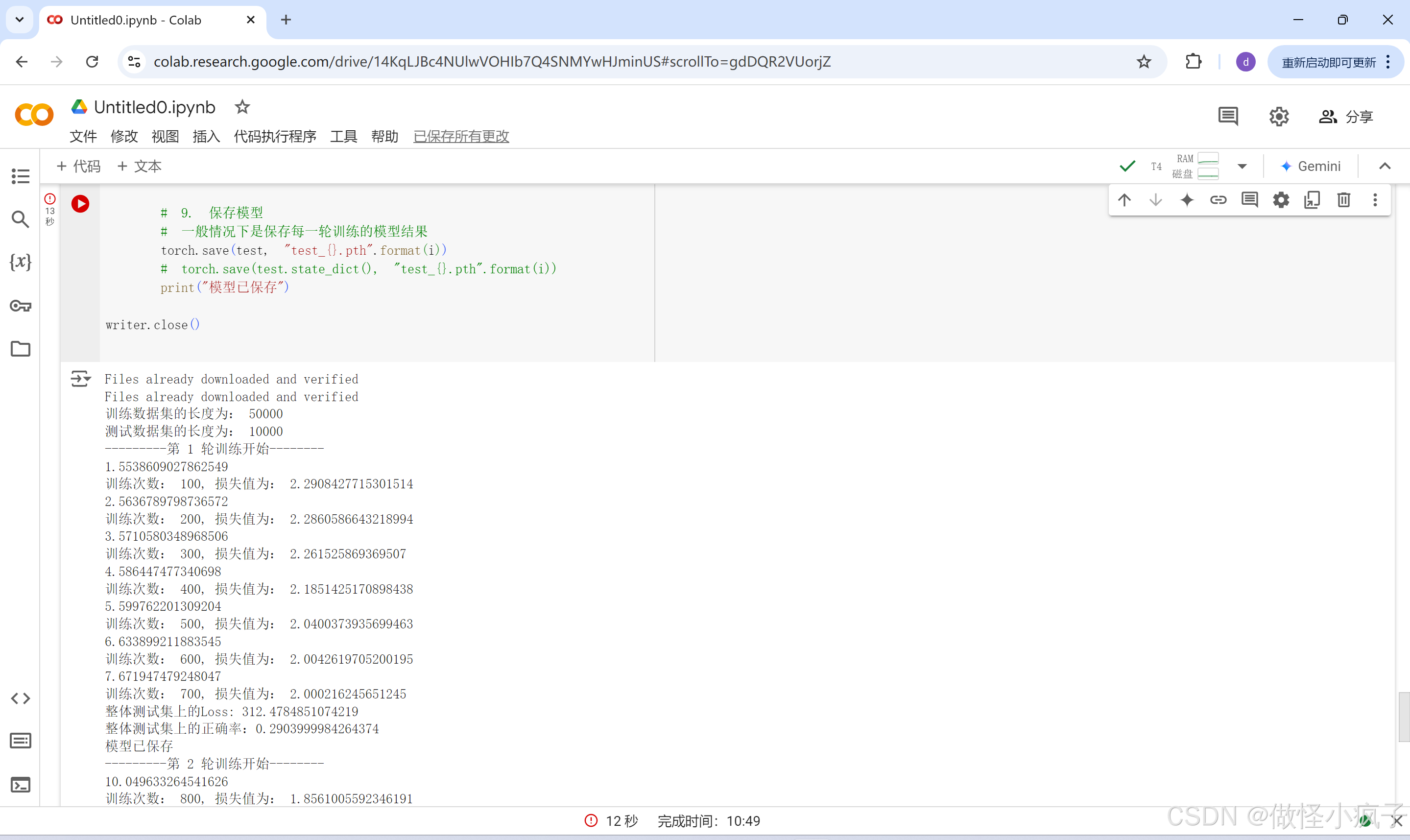
9. 保存模型
# 一般情况下是保存每一轮训练的模型结果
    torch.save(test, "test_{}.pth".format(i))
    # torch.save(test.state_dict(), "test_{}.pth".format(i))
    print("模型已保存")
总体代码如下:
import torch
import torchvision
from torch import nn
from torch.nn import Sequential, Conv2d, MaxPool2d, Flatten, Linear
from torch.utils.data import DataLoader
from torch.utils.tensorboard import SummaryWriter
from model import *

# 1.准备数据集
train_data = torchvision.datasets.CIFAR10('./CIFAR10', train=True, transform=torchvision.transforms.ToTensor(),
                                          download=True)

test_data = torchvision.datasets.CIFAR10('./CIFAR10', train=False, transform=torchvision.transforms.ToTensor(),
                                         download=True)

# 获得数据集的长度
train_data_size = len(train_data)
test_data_size = len(test_data)
# 格式化字符串的方式
print("训练数据集的长度为: {}".format(train_data_size)) # 50000
print("测试数据集的长度为: {}".format(test_data_size)) # 10000

# 2.利用dataloader加载数据集
train_dataloader = DataLoader(train_data, batch_size=64)
test_dataloader = DataLoader(test_data, batch_size=64)

# 3.创建网络模型
test = Test()

# 4.创建损失函数
loss_function = nn.CrossEntropyLoss()

# 5.创建优化器
# learning_rate = 0.01
learning_rate = 1e-2 # 1e-2 = 10^(-2)
optimizer = torch.optim.SGD(test.parameters(), lr=learning_rate)

# 6.设置训练网络的一些参数
# 记录训练的次数:
total_train_step = 0
# 记录测试的次数:
total_test_step = 0

# 记录训练的轮数:
epoch = 10

# 使用tensorboard
writer = SummaryWriter("./logs_train")

# 7.设置训练轮数、开始训练
for i in range(epoch):
    print("---------第 {} 轮训练开始--------".format(i + 1))
    # 训练开始:
    test.train() # 将网络设置为训练模式,只对某些特定的网络有作用,比如当网络中有Dropout、BatchNorm层等的时候
    for data in train_dataloader:
        imgs, targets = data
        outputs = test(imgs)
        # 记录损失
        loss = loss_function(outputs, targets)
        # 优化器优化模型
        optimizer.zero_grad() # 梯度清零
        loss.backward() # 梯度下降
        optimizer.step() # 对每个梯度进行优化

        total_train_step = total_train_step + 1
        # item():将tensor类型转为实际的值
        if (total_train_step % 100 == 0):
            print("训练次数: {}, 损失值为: {}".format(total_train_step, loss.item()))
            writer.add_scalar("train_loss", loss.item(),  total_train_step)

    # 8. 测试模型
    # 如何知道模型有没有训练好---------进行测试,在测试集上跑一遍,用测试数据集上的损失或正确率来评估模型有没有训练好
    # 测试步骤:
    test.eval() # 将网络模式设置为测试状态,也是只对特定的网络有作用,比如当网络中有Dropout、BatchNorm层等的时候
    total_test_loss = 0
    total_accuracy = 0
    test.eval()
    with torch.no_grad():# 将网络模型中的梯度消失,只需要测试,不需要对梯度进行调整,也不需要利用梯度来优化
        for data in test_dataloader:
            imgs, targets = data
            outputs = test(imgs)
            loss = loss_function(outputs, targets)
            total_test_loss += loss
            # 正确率
            accuracy = (outputs.argmax(1) == targets).sum()
            total_accuracy = total_accuracy + accuracy
    # 使用一些参数,比如损失函数和正确率来展示网络训练的效果(正确率一般分类问题中经常使用)
    print("整体测试集上的Loss: {}".format(total_test_loss))
    print("整体测试集上的正确率:{}".format(total_accuracy / test_data_size))
    writer.add_scalar("test_loss", total_test_loss, total_test_step)
    writer.add_scalar("test_accuracy", total_accuracy, total_test_step)
    total_test_step += 1

    # 9. 保存模型
    # 一般情况下是保存每一轮训练的模型结果
    torch.save(test, "test_{}.pth".format(i))
    # torch.save(test.state_dict(), "test_{}.pth".format(i))
    print("模型已保存")
利用GPU训练
利用GPU训练方式1
找到网络模型、数据(输入、标注)、损失函数;在后面添加.cuda(),例如:
test = Test()
if torch.cuda.is_available(): # 这样写也可以
    test = test.cuda()
注意:数据是指在训练网络进行读取数据的时候设置的。
for data in train_data_loader:
	imgs, targets = data
        if torch.cuda.is_available():
            imgs = imgs.cuda()
            targets = targets.cuda()
....
完整代码如下:
import time

import torch
import torchvision
from torch import nn
from torch.nn import Sequential, Conv2d, MaxPool2d, Flatten, Linear
from torch.utils.data import DataLoader
from torch.utils.tensorboard import SummaryWriter
# from model import *

# 1.准备数据集
train_data = torchvision.datasets.CIFAR10('./CIFAR10', train=True, transform=torchvision.transforms.ToTensor(),
                                          download=True)

test_data = torchvision.datasets.CIFAR10('./CIFAR10', train=False, transform=torchvision.transforms.ToTensor(),
                                         download=True)

# 获得数据集的长度
train_data_size = len(train_data)
test_data_size = len(test_data)
# 格式化字符串的方式
print("训练数据集的长度为: {}".format(train_data_size)) # 50000
print("测试数据集的长度为: {}".format(test_data_size)) # 10000

# 2.利用dataloader加载数据集
train_dataloader = DataLoader(train_data, batch_size=64)
test_dataloader = DataLoader(test_data, batch_size=64)

# 3.创建网络模型
class Test(nn.Module):
    def __init__(self):
        super(Test, self).__init__()
        self.model = nn.Sequential(
            nn.Conv2d(3, 32, 5, 1, 2),
            nn.MaxPool2d(2),
            nn.Conv2d(32, 32, 5, 1, 2),
            nn.MaxPool2d(2),
            nn.Conv2d(32, 64, 5, 1, 2),
            nn.MaxPool2d(2),
            nn.Flatten(),
            nn.Linear(64 * 4 * 4, 64),
            nn.Linear(64, 10)
        )

    def forward(self, x):
        x = self.model(x)
        return x
test = Test()
if torch.cuda.is_available():
    test = test.cuda()

# 4.创建损失函数
loss_function = nn.CrossEntropyLoss()
if torch.cuda.is_available():
    loss_function = loss_function.cuda()

# 5.创建优化器
# learning_rate = 0.01
learning_rate = 1e-2 # 1e-2 = 10^(-2)
optimizer = torch.optim.SGD(test.parameters(), lr=learning_rate)

# 6.设置训练网络的一些参数
# 记录训练的次数:
total_train_step = 0
# 记录测试的次数:
total_test_step = 0

# 记录训练的轮数:
epoch = 10

# 使用tensorboard
writer = SummaryWriter("./logs_train")
start_time = time.time()
# 7.设置训练轮数、开始训练
for i in range(epoch):
    print("---------第 {} 轮训练开始--------".format(i + 1))
    # 训练开始:
    test.train() # 将网络设置为训练模式,只对某些特定的网络有作用,比如当网络中有Dropout、BatchNorm层等的时候
    for data in train_dataloader:
        imgs, targets = data
        if torch.cuda.is_available():
            imgs = imgs.cuda()
            targets = targets.cuda()
        outputs = test(imgs)
        # 记录损失
        loss = loss_function(outputs, targets)
        # 优化器优化模型
        optimizer.zero_grad() # 梯度清零
        loss.backward() # 梯度下降
        optimizer.step() # 对每个梯度进行优化

        total_train_step = total_train_step + 1
        # item():将tensor类型转为实际的值
        if (total_train_step % 100 == 0):
            end_time = time.time()
            print(end_time - start_time)
            print("训练次数: {}, 损失值为: {}".format(total_train_step, loss.item()))
            writer.add_scalar("train_loss", loss.item(),  total_train_step)

    # 8. 测试模型
    # 如何知道模型有没有训练好---------进行测试,在测试集上跑一遍,用测试数据集上的损失或正确率来评估模型有没有训练好
    # 测试步骤:
    test.eval() # 将网络模式设置为测试状态,也是只对特定的网络有作用,比如当网络中有Dropout、BatchNorm层等的时候
    total_test_loss = 0
    total_accuracy = 0
    test.eval()
    with torch.no_grad():# 将网络模型中的梯度消失,只需要测试,不需要对梯度进行调整,也不需要利用梯度来优化
        for data in test_dataloader:
            imgs, targets = data
            if torch.cuda.is_available():
                imgs = imgs.cuda()
                targets = targets.cuda()
            outputs = test(imgs)
            loss = loss_function(outputs, targets)
            total_test_loss += loss
            # 正确率
            accuracy = (outputs.argmax(1) == targets).sum()
            total_accuracy = total_accuracy + accuracy
    # 使用一些参数,比如损失函数和正确率来展示网络训练的效果(正确率一般分类问题中经常使用)
    print("整体测试集上的Loss: {}".format(total_test_loss))
    print("整体测试集上的正确率:{}".format(total_accuracy / test_data_size))
    writer.add_scalar("test_loss", total_test_loss, total_test_step)
    writer.add_scalar("test_accuracy", total_accuracy, total_test_step)
    total_test_step += 1

    # 9. 保存模型
    # 一般情况下是保存每一轮训练的模型结果
    torch.save(test, "test_{}.pth".format(i))
    # torch.save(test.state_dict(), "test_{}.pth".format(i))
    print("模型已保存")

writer.close()
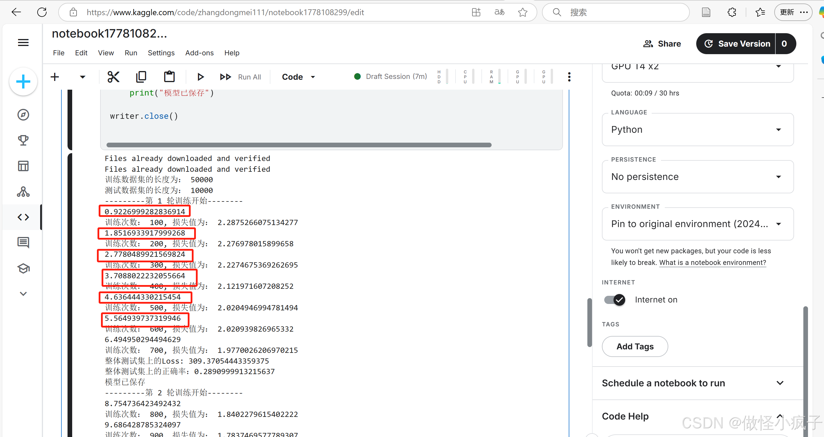
cpu上的运行结果:
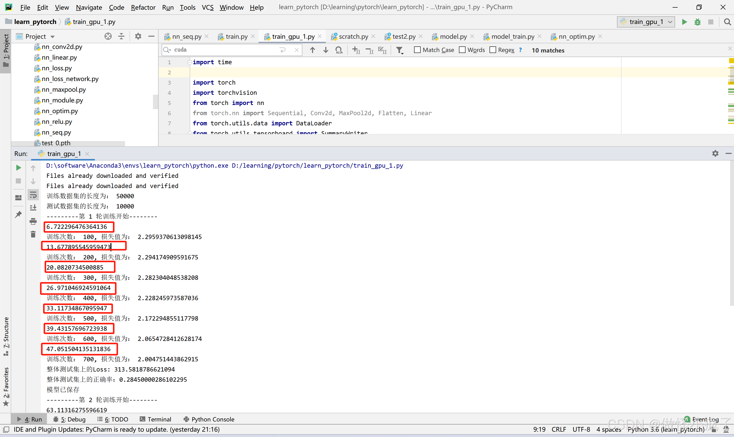
由于我电脑不支持gpu的使用,因此我将代码复制到了kaggle上进行了一个运行,可以看到运行时间比在cpu上的运行时间提高了6-7倍。
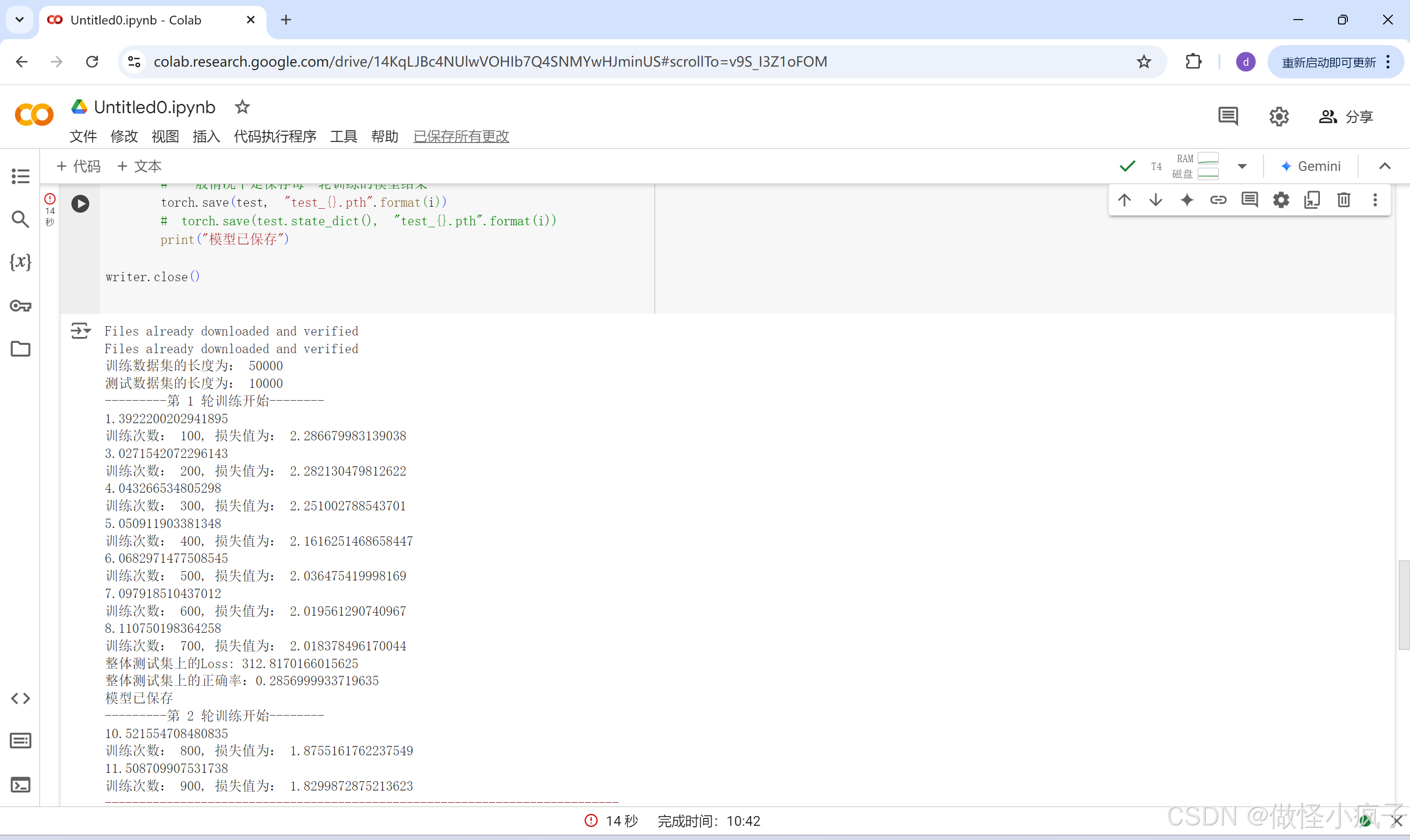
使用博主推荐的colal上进行运行,可得到如下的运行结果,也是比较快的。。
利用GPU训练的另一种方式
使用.to(device), 其中device = torch.device("cpu")。例如:
torch.device("cuda")
torch.device("cuda:0") # 第一张显卡
torch.device("cuda:1") # 第二张显卡
修改代码为:
import time

import torch
import torchvision
from torch import nn
from torch.nn import Sequential, Conv2d, MaxPool2d, Flatten, Linear
from torch.utils.data import DataLoader
from torch.utils.tensorboard import SummaryWriter
# from model import *

# 定义训练的设备
device = torch.device("cuda")
# 1.准备数据集
train_data = torchvision.datasets.CIFAR10('./CIFAR10', train=True, transform=torchvision.transforms.ToTensor(),
                                          download=True)

test_data = torchvision.datasets.CIFAR10('./CIFAR10', train=False, transform=torchvision.transforms.ToTensor(),
                                         download=True)

# 获得数据集的长度
train_data_size = len(train_data)
test_data_size = len(test_data)
# 格式化字符串的方式
print("训练数据集的长度为: {}".format(train_data_size)) # 50000
print("测试数据集的长度为: {}".format(test_data_size)) # 10000

# 2.利用dataloader加载数据集
train_dataloader = DataLoader(train_data, batch_size=64)
test_dataloader = DataLoader(test_data, batch_size=64)

# 3.创建网络模型
class Test(nn.Module):
    def __init__(self):
        super(Test, self).__init__()
        self.model = nn.Sequential(
            nn.Conv2d(3, 32, 5, 1, 2),
            nn.MaxPool2d(2),
            nn.Conv2d(32, 32, 5, 1, 2),
            nn.MaxPool2d(2),
            nn.Conv2d(32, 64, 5, 1, 2),
            nn.MaxPool2d(2),
            nn.Flatten(),
            nn.Linear(64 * 4 * 4, 64),
            nn.Linear(64, 10)
        )

    def forward(self, x):
        x = self.model(x)
        return x
test = Test()
# if torch.cuda.is_available():
#     test = test.cuda()
test.to(device)

# 4.创建损失函数
loss_function = nn.CrossEntropyLoss()
# if torch.cuda.is_available():
#     loss_function = loss_function.cuda()
loss_function.to(device)

# 5.创建优化器
# learning_rate = 0.01
learning_rate = 1e-2 # 1e-2 = 10^(-2)
optimizer = torch.optim.SGD(test.parameters(), lr=learning_rate)

# 6.设置训练网络的一些参数
# 记录训练的次数:
total_train_step = 0
# 记录测试的次数:
total_test_step = 0

# 记录训练的轮数:
epoch = 10

# 使用tensorboard
writer = SummaryWriter("./logs_train")
start_time = time.time()
# 7.设置训练轮数、开始训练
for i in range(epoch):
    print("---------第 {} 轮训练开始--------".format(i + 1))
    # 训练开始:
    test.train() # 将网络设置为训练模式,只对某些特定的网络有作用,比如当网络中有Dropout、BatchNorm层等的时候
    for data in train_dataloader:
        imgs, targets = data
        # if torch.cuda.is_available():
        #     imgs = imgs.cuda()
        #     targets = targets.cuda()
        imgs = imgs.to(device)
        targets = targets.to(device)
        outputs = test(imgs)
        # 记录损失
        loss = loss_function(outputs, targets)
        # 优化器优化模型
        optimizer.zero_grad() # 梯度清零
        loss.backward() # 梯度下降
        optimizer.step() # 对每个梯度进行优化

        total_train_step = total_train_step + 1
        # item():将tensor类型转为实际的值
        if (total_train_step % 100 == 0):
            end_time = time.time()
            print(end_time - start_time)
            print("训练次数: {}, 损失值为: {}".format(total_train_step, loss.item()))
            writer.add_scalar("train_loss", loss.item(),  total_train_step)

    # 8. 测试模型
    # 如何知道模型有没有训练好---------进行测试,在测试集上跑一遍,用测试数据集上的损失或正确率来评估模型有没有训练好
    # 测试步骤:
    test.eval() # 将网络模式设置为测试状态,也是只对特定的网络有作用,比如当网络中有Dropout、BatchNorm层等的时候
    total_test_loss = 0
    total_accuracy = 0
    test.eval()
    with torch.no_grad():# 将网络模型中的梯度消失,只需要测试,不需要对梯度进行调整,也不需要利用梯度来优化
        for data in test_dataloader:
            imgs, targets = data
            # if torch.cuda.is_available():
            #     imgs = imgs.cuda()
            #     targets = targets.cuda()
            imgs = imgs.to(device)
            targets = targets.to(device)
            outputs = test(imgs)
            loss = loss_function(outputs, targets)
            total_test_loss += loss
            # 正确率
            accuracy = (outputs.argmax(1) == targets).sum()
            total_accuracy = total_accuracy + accuracy
    # 使用一些参数,比如损失函数和正确率来展示网络训练的效果(正确率一般分类问题中经常使用)
    print("整体测试集上的Loss: {}".format(total_test_loss))
    print("整体测试集上的正确率:{}".format(total_accuracy / test_data_size))
    writer.add_scalar("test_loss", total_test_loss, total_test_step)
    writer.add_scalar("test_accuracy", total_accuracy, total_test_step)
    total_test_step += 1

    # 9. 保存模型
    # 一般情况下是保存每一轮训练的模型结果
    torch.save(test, "test_{}.pth".format(i))
    # torch.save(test.state_dict(), "test_{}.pth".format(i))
    print("模型已保存")
writer.close()
结果如下:
注意:模型、损失函数不需要另外赋值,即model.to(device)即可,而数据(输入、标注)需要赋值。方便记忆:可以都进行赋值。
对于单显卡,以下两种写法没有区别:
device = torch.device("cuda")
devide = torch.device("cuda:0")
也有人这样写:
devide = torch.device("cuda" if torch.cuda.is_avaliable() else "cpu")
完整的模型验证套路
核心:利用已经训练好的模型,然后给它提供输入。
完整代码:
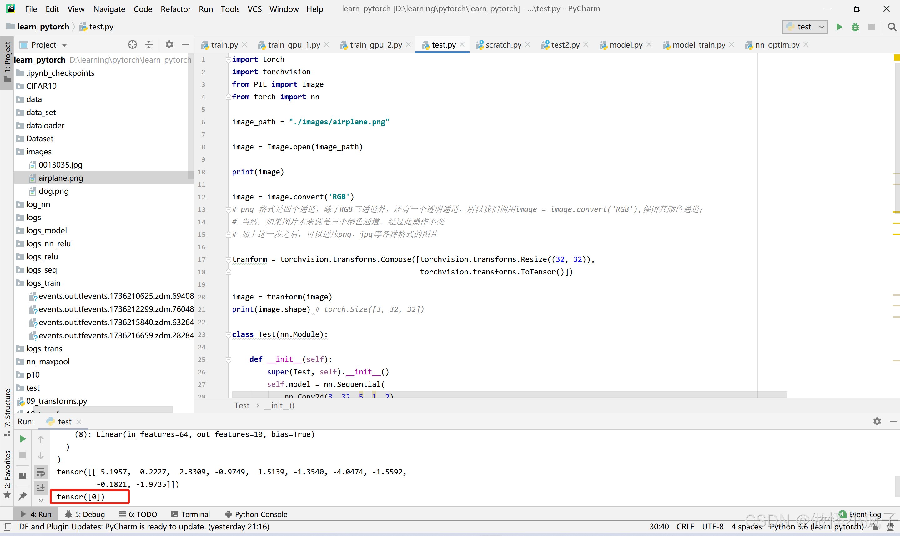
import torch
import torchvision
from PIL import Image
from torch import nn

image_path = "./images/airplane.png"

image = Image.open(image_path)

print(image)

image = image.convert('RGB')
# png 格式是四个通道,除了RGB三通道外,还有一个透明通道,所以我们调用image = image.convert('RGB'),保留其颜色通道;
# 当然,如果图片本来就是三个颜色通道,经过此操作不变
# 加上这一步之后,可以适应png、jpg等各种格式的图片

tranform = torchvision.transforms.Compose([torchvision.transforms.Resize((32, 32)),
                                           torchvision.transforms.ToTensor()])

image = tranform(image)
print(image.shape) # torch.Size([3, 32, 32])

class Test(nn.Module):

    def __init__(self):
        super(Test, self).__init__()
        self.model = nn.Sequential(
            nn.Conv2d(3, 32, 5, 1, 2),
            nn.MaxPool2d(2),
            nn.Conv2d(32, 32, 5, 1, 2),
            nn.MaxPool2d(2),
            nn.Conv2d(32, 64, 5, 1, 2),
            nn.MaxPool2d(2),
            nn.Flatten(),
            nn.Linear(64 * 4 * 4, 64),
            nn.Linear(64, 10)
        )

    def forward(self, x):
        x = self.model(x)
        return x

# 直接加载会报错: Attempting to deserialize object on a CUDA device but torch.cuda.is_available() is False. If you are running on a CPU-only machine, please use torch.load with
# 需要添加参数:map_location=torch.device('cpu')
model = torch.load("test_9_gpu.pth", map_location=torch.device('cpu'))
print(model)
# Expected 4-dimensional input for 4-dimensional weight [32, 3, 5, 5], but got 3-dimensional input of size [3, 32, 32] instead
# 解决:
image = torch.reshape(image, (1, 3, 32, 32))
model.eval()
with torch.no_grad():
    output = model(image)
print(output)
# 结果:
print(output.argmax(1))
我使用了一张飞机的图片,结果如下所示:
kaggle&colab gpu使用
kaggle为每位用户提供每周30h的免费GPU使用时间。目前我电脑没有gpu,因此,想先用着这上面的先进行学习吧。
【最后】总结
可以尝试看一些开源项目。平时学习的时候可以多看官方文档,多多练习,目前感觉算是入门啦,非常感谢up主。


 被折叠的 条评论
为什么被折叠?
被折叠的 条评论
为什么被折叠?
 到【灌水乐园】发言


