


- 🍨 本文为🔗365天深度学习训练营 中的学习记录博客
- 🍖 原作者:K同学啊
👉 学习目标:
●
学习使用LSTM对糖尿病进行探索预测
●
本文的预测准确率,请尝试将其提升到70%以上(下一周更新我的解决方案)
1数据预处理
1.1设置GPU
import torch.nn as nn
import torch.nn.functional as F
import torchvision,torch

# 设置硬件设备,如果有GPU则使用,没有则使用cpu
device = torch.device("cuda" if torch.cuda.is_available() else "cpu")
device
1.2数据导入
import numpy             as np
import pandas            as pd
import seaborn           as sns
from sklearn.model_selection   import train_test_split
import matplotlib.pyplot as plt
plt.rcParams['savefig.dpi'] = 500 #图片像素
plt.rcParams['figure.dpi']  = 500 #分辨率

plt.rcParams['font.sans-serif'] = ['SimHei']  # 用来正常显示中文标签

import warnings
warnings.filterwarnings("ignore")

DataFrame=pd.read_excel(r'/home/aiusers/space_yjl/深度学习训练营/进阶/第R6周:LSTM实现糖尿病探索与预测/dia.xls')
DataFrame.head()
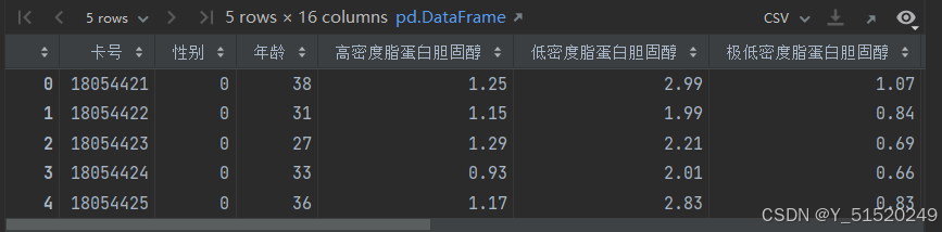
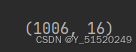
DataFrame.shape
1.3数据检查
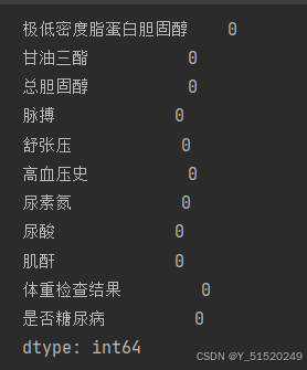
# 查看数据是否有缺失值
print('数据缺失值---------------------------------')
print(DataFrame.isnull().sum())
# 查看数据是否有重复值
print('数据重复值---------------------------------')
print('数据集的重复值为:'f'{DataFrame.duplicated().sum()}')
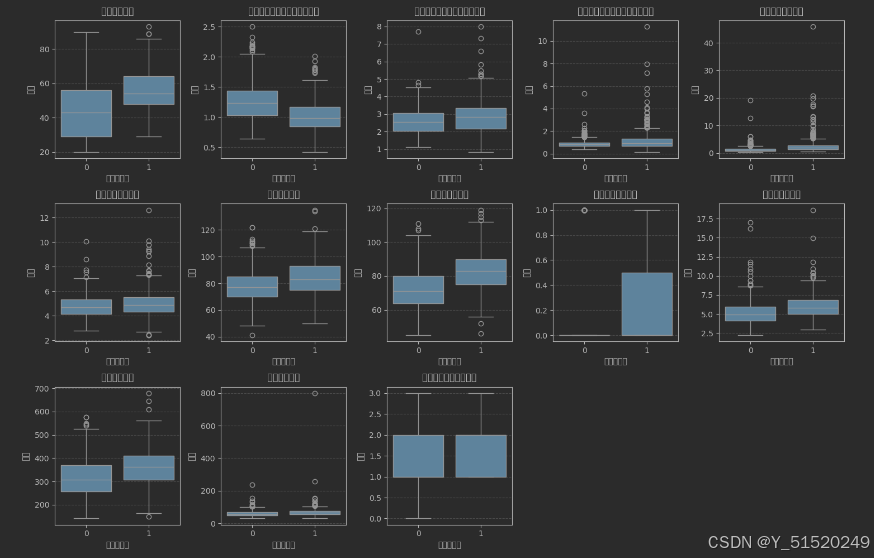
1.4数据分布分析
feature_map = {
    '年龄': '年龄',
    '高密度脂蛋白胆固醇': '高密度脂蛋白胆固醇',
    '低密度脂蛋白胆固醇': '低密度脂蛋白胆固醇',
    '极低密度脂蛋白胆固醇': '极低密度脂蛋白胆固醇',
    '甘油三酯': '甘油三酯',
    '总胆固醇': '总胆固醇',
    '脉搏': '脉搏',
    '舒张压':'舒张压',
    '高血压史':'高血压史',
    '尿素氮':'尿素氮',
    '尿酸':'尿酸',
    '肌酐':'肌酐',
    '体重检查结果':'体重检查结果'
}
plt.figure(figsize=(15, 10))

for i, (col, col_name) in enumerate(feature_map.items(), 1):
    plt.subplot(3, 5, i)
    sns.boxplot(x=DataFrame['是否糖尿病'], y=DataFrame[col])
    plt.title(f'{col_name}的箱线图', fontsize=14)
    plt.ylabel('数值', fontsize=12)
    plt.grid(axis='y', linestyle='--', alpha=0.7)

plt.tight_layout()
plt.show()
这个因为或者环境的问题,导致图片不能正常可视化 后续会补充解决的。
2.LSTM 模型
2.1数据集构建
from sklearn.preprocessing import StandardScaler

# '高密度脂蛋白胆固醇'字段与糖尿病负相关,故而在 X 中去掉该字段
X = DataFrame.drop(['卡号','是否糖尿病','高密度脂蛋白胆固醇'],axis=1)
y = DataFrame['是否糖尿病']

# sc_X    = StandardScaler()
# X = sc_X.fit_transform(X)

X = torch.tensor(np.array(X), dtype=torch.float32)
y = torch.tensor(np.array(y), dtype=torch.int64)

train_X, test_X, train_y, test_y = train_test_split(X, y,
                                                    test_size=0.2,
                                                    random_state=1)
train_X.shape, train_y.shape

from torch.utils.data import TensorDataset, DataLoader

train_dl = DataLoader(TensorDataset(train_X, train_y),
                      batch_size=64,
                      shuffle=False)

test_dl  = DataLoader(TensorDataset(test_X, test_y),
                      batch_size=64,
                      shuffle=False)
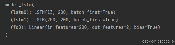
2.2定义模型
class model_lstm(nn.Module):
    def __init__(self):
        super(model_lstm, self).__init__()
        self.lstm0 = nn.LSTM(input_size=13 ,hidden_size=200,
                             num_layers=1, batch_first=True)

        self.lstm1 = nn.LSTM(input_size=200 ,hidden_size=200,
                             num_layers=1, batch_first=True)
        self.fc0   = nn.Linear(200, 2)

    def forward(self, x):

        out, hidden1 = self.lstm0(x)
        out, _ = self.lstm1(out, hidden1)
        out    = self.fc0(out)
        return out

model = model_lstm().to(device)
model
3.训练模型
3.1定义训练函数
# 训练循环
def train(dataloader, model, loss_fn, optimizer):
    size = len(dataloader.dataset)  # 训练集的大小
    num_batches = len(dataloader)   # 批次数目, (size/batch_size,向上取整)

    train_loss, train_acc = 0, 0  # 初始化训练损失和正确率

    for X, y in dataloader:  # 获取图片及其标签
        X, y = X.to(device), y.to(device)

        # 计算预测误差
        pred = model(X)          # 网络输出
        loss = loss_fn(pred, y)  # 计算网络输出和真实值之间的差距,targets为真实值,计算二者差值即为损失

        # 反向传播
        optimizer.zero_grad()  # grad属性归零
        loss.backward()        # 反向传播
        optimizer.step()       # 每一步自动更新

        # 记录acc与loss
        train_acc  += (pred.argmax(1) == y).type(torch.float).sum().item()
        train_loss += loss.item()

    train_acc  /= size
    train_loss /= num_batches

    return train_acc, train_loss
3.2定义测试函数
def test (dataloader, model, loss_fn):
    size        = len(dataloader.dataset)  # 测试集的大小
    num_batches = len(dataloader)          # 批次数目, (size/batch_size,向上取整)
    test_loss, test_acc = 0, 0

    # 当不进行训练时,停止梯度更新,节省计算内存消耗
    with torch.no_grad():
        for imgs, target in dataloader:
            imgs, target = imgs.to(device), target.to(device)

            # 计算loss
            target_pred = model(imgs)
            loss        = loss_fn(target_pred, target)

            test_loss += loss.item()
            test_acc  += (target_pred.argmax(1) == target).type(torch.float).sum().item()

    test_acc  /= size
    test_loss /= num_batches

    return test_acc, test_loss
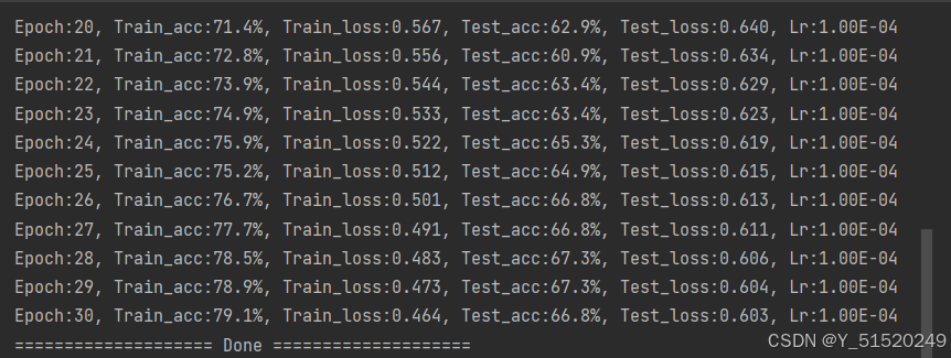
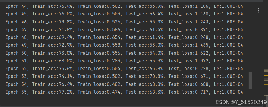
3.3训练模型
loss_fn    = nn.CrossEntropyLoss() # 创建损失函数
learn_rate = 1e-4   # 学习率
opt        = torch.optim.Adam(model.parameters(),lr=learn_rate)
epochs     = 30

train_loss = []
train_acc  = []
test_loss  = []
test_acc   = []

for epoch in range(epochs):
    model.train()
    epoch_train_acc, epoch_train_loss = train(train_dl, model, loss_fn, opt)

    model.eval()
    epoch_test_acc, epoch_test_loss = test(test_dl, model, loss_fn)

    train_acc.append(epoch_train_acc)
    train_loss.append(epoch_train_loss)
    test_acc.append(epoch_test_acc)
    test_loss.append(epoch_test_loss)

    # 获取当前的学习率
    lr = opt.state_dict()['param_groups'][0]['lr']

    template = ('Epoch:{:2d}, Train_acc:{:.1f}%, Train_loss:{:.3f}, Test_acc:{:.1f}%, Test_loss:{:.3f}, Lr:{:.2E}')
    print(template.format(epoch+1, epoch_train_acc*100, epoch_train_loss,
                          epoch_test_acc*100, epoch_test_loss, lr))

print("="*20, 'Done', "="*20)
4模型评估
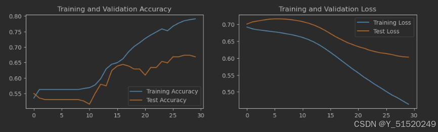
4.1Loss与Accuracy图
import matplotlib.pyplot as plt
#隐藏警告
import warnings
warnings.filterwarnings("ignore")               #忽略警告信息
plt.rcParams['font.sans-serif']    = ['SimHei'] # 用来正常显示中文标签
plt.rcParams['axes.unicode_minus'] = False      # 用来正常显示负号
plt.rcParams['figure.dpi']         = 100        #分辨率

epochs_range = range(epochs)

plt.figure(figsize=(12, 3))
plt.subplot(1, 2, 1)

plt.plot(epochs_range, train_acc, label='Training Accuracy')
plt.plot(epochs_range, test_acc, label='Test Accuracy')
plt.legend(loc='lower right')
plt.title('Training and Validation Accuracy')

plt.subplot(1, 2, 2)
plt.plot(epochs_range, train_loss, label='Training Loss')
plt.plot(epochs_range, test_loss, label='Test Loss')
plt.legend(loc='upper right')
plt.title('Training and Validation Loss')
plt.show()
5.个人总结
通过结合多层 LSTM 网络、残差连接、以及注意力机制(Attention),提高对序列数据的建模能力。
import torch
import torch.nn as nn

class EnhancedLSTM(nn.Module):
    def __init__(self):
        super(EnhancedLSTM, self).__init__()
        # 第一层 LSTM
        self.lstm0 = nn.LSTM(input_size=13, hidden_size=256,
                             num_layers=2, batch_first=True, dropout=0.2)
        # 第二层 LSTM
        self.lstm1 = nn.LSTM(input_size=256, hidden_size=256,
                             num_layers=2, batch_first=True, dropout=0.2)
        # 残差连接的全连接层
        self.fc_residual = nn.Linear(13, 256)
        # Attention 层
        self.attention = nn.Linear(256, 1)
        # 最后的全连接层
        self.fc0 = nn.Linear(256, 2)

    def forward(self, x):
        # 残差连接
        residual = self.fc_residual(x)
        # 第一层 LSTM
        out, _ = self.lstm0(x)
        # 第二层 LSTM
        out, _ = self.lstm1(out)
        # 添加残差
        out = out + residual
        # 确保 out 是三维张量 (batch_size, sequence_length, hidden_size)
        if out.dim() == 2:
            out = out.unsqueeze(1)  # 增加一个时间步维度 (batch_size, 1, hidden_size)
        # 选择最后一个时间步的输出
        out = out[:, -1, :]  # (batch_size, hidden_size)
        # Attention 机制
        attn_weights = torch.softmax(self.attention(out.unsqueeze(1)), dim=1)
        out = torch.sum(attn_weights * out.unsqueeze(1), dim=1)
        # 输出层
        out = self.fc0(out)
        return out

# 设备选择
device = torch.device("cuda" if torch.cuda.is_available() else "cpu")
model = EnhancedLSTM().to(device)
print(model)
关键特点:
多层 LSTM:
通过多层的 LSTM 网络,模型能够更好地捕捉序列中的长程依赖关系。
残差连接:
残差连接有助于缓解深层网络中的梯度消失问题,使得信息在网络中能够更好地传递。
注意力机制:
通过引入注意力机制,模型能够根据输入序列的不同部分赋予不同的权重,从而提升对关键信息的捕捉能力。
灵活的输入处理:
如果 out 的维度被压缩为二维,模型会通过 unsqueeze(1) 将其转换回三维,确保可以处理不同形状的输入。


 1110
1110

 被折叠的 条评论
为什么被折叠?
被折叠的 条评论
为什么被折叠?
 到【灌水乐园】发言


