


- 🍨 本文为🔗365天深度学习训练营 中的学习记录博客
- 🍖 原作者:K同学啊
一、前期工作
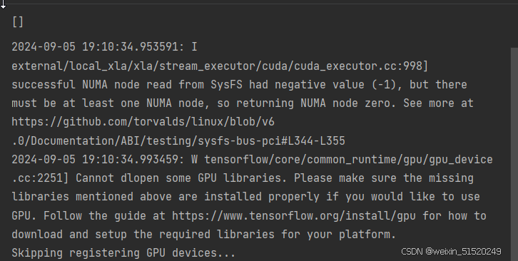
1. 设置GPU
如果使用的是CPU可以注释掉这部分的代码。
import tensorflow as tf

gpus = tf.config.list_physical_devices("GPU")

if gpus:
    tf.config.experimental.set_memory_growth(gpus[0], True)  #设置GPU显存用量按需使用
    tf.config.set_visible_devices([gpus[0]],"GPU")

# 打印显卡信息,确认GPU可用
print(gpus)
2. 导入数据
import matplotlib.pyplot as plt
# 支持中文
plt.rcParams['font.sans-serif'] = ['SimHei']  # 用来正常显示中文标签
plt.rcParams['axes.unicode_minus'] = False  # 用来正常显示负号

import os,PIL,pathlib

#隐藏警告
import warnings
warnings.filterwarnings('ignore')

data_dir = "/home/aiusers/space_yjl/深度学习训练营/Tensorflow入门实战/第八周:猫狗识别/365-7-data"
data_dir = pathlib.Path(data_dir)

image_count = len(list(data_dir.glob('*/*')))

print("图片总数为:",image_count)
二、数据预处理
1. 加载数据
使用image_dataset_from_directory方法将磁盘中的数据加载到tf.data.Dataset中
batch_size = 8
img_height = 224
img_width = 224
"""
关于image_dataset_from_directory()的详细介绍可以参考文章:https://mtyjkh.blog.youkuaiyun.com/article/details/117018789
"""
train_ds = tf.keras.preprocessing.image_dataset_from_directory(
    data_dir,
    validation_split=0.2,
    subset="training",
    seed=12,
    image_size=(img_height, img_width),
    batch_size=batch_size)
"""
关于image_dataset_from_directory()的详细介绍可以参考文章:https://mtyjkh.blog.youkuaiyun.com/article/details/117018789
"""
val_ds = tf.keras.preprocessing.image_dataset_from_directory(
    data_dir,
    validation_split=0.2,
    subset="validation",
    seed=12,
    image_size=(img_height, img_width),
    batch_size=batch_size)
我们可以通过class_names输出数据集的标签。标签将按字母顺序对应于目录名称。
class_names = train_ds.class_names
print(class_names)
2. 再次检查数据
for image_batch, labels_batch in train_ds:
    print(image_batch.shape)
    print(labels_batch.shape)
    break
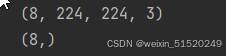
● Image_batch是形状的张量(8, 224, 224, 3)。这是一批形状224x224x3的8张图片(最后一维指的是彩色通道RGB)。
● Label_batch是形状(8,)的张量,这些标签对应8张图片
3. 配置数据集
● shuffle() : 打乱数据,关于此函数的详细介绍可以参考:https://zhuanlan.zhihu.com/p/42417456
● prefetch() :预取数据,加速运行,其详细介绍可以参考我前两篇文章,里面都有讲解。
● cache() :将数据集缓存到内存当中,加速运行
AUTOTUNE = tf.data.AUTOTUNE

def preprocess_image(image,label):
    return (image/255.0,label)

# 归一化处理
train_ds = train_ds.map(preprocess_image, num_parallel_calls=AUTOTUNE)
val_ds   = val_ds.map(preprocess_image, num_parallel_calls=AUTOTUNE)

train_ds = train_ds.cache().shuffle(1000).prefetch(buffer_size=AUTOTUNE)
val_ds   = val_ds.cache().prefetch(buffer_size=AUTOTUNE)
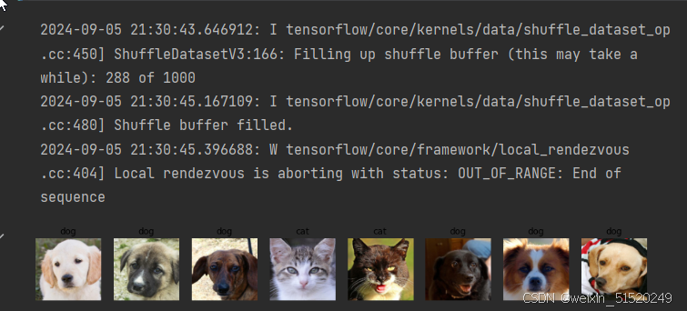
4. 可视化数据
plt.figure(figsize=(15, 10))  # 图形的宽为15高为10

for images, labels in train_ds.take(1):
    for i in range(8):

        ax = plt.subplot(5, 8, i + 1)
        plt.imshow(images[i])
        plt.title(class_names[labels[i]])

        plt.axis("off")
三、构建VG-16网络
VGG优缺点分析:
● VGG优点
VGG的结构非常简洁,整个网络都使用了同样大小的卷积核尺寸(3x3)和最大池化尺寸(2x2)。
● VGG缺点
1)训练时间过长,调参难度大。2)需要的存储容量大,不利于部署。例如存储VGG-16权重值文件的大小为500多MB,不利于安装到嵌入式系统中。
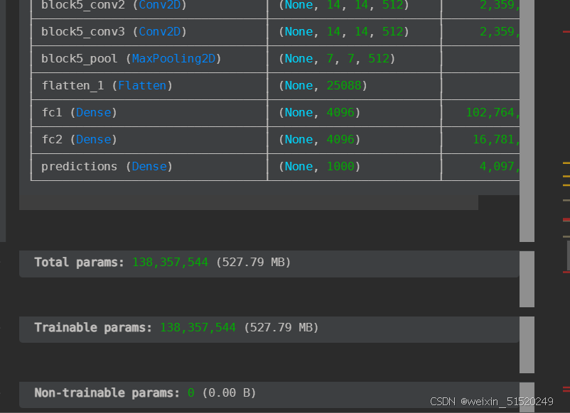
结构说明:
● 13个卷积层(Convolutional Layer),分别用blockX_convX表示
● 3个全连接层(Fully connected Layer),分别用fcX与predictions表示
● 5个池化层(Pool layer),分别用blockX_pool表示
VGG-16包含了16个隐藏层(13个卷积层和3个全连接层),故称为VGG-16
from tensorflow.keras import layers, models, Input
from tensorflow.keras.models import Model
from tensorflow.keras.layers import Conv2D, MaxPooling2D, Dense, Flatten, Dropout

def VGG16(nb_classes, input_shape):
    input_tensor = Input(shape=input_shape)
    # 1st block
    x = Conv2D(64, (3,3), activation='relu', padding='same',name='block1_conv1')(input_tensor)
    x = Conv2D(64, (3,3), activation='relu', padding='same',name='block1_conv2')(x)
    x = MaxPooling2D((2,2), strides=(2,2), name = 'block1_pool')(x)
    # 2nd block
    x = Conv2D(128, (3,3), activation='relu', padding='same',name='block2_conv1')(x)
    x = Conv2D(128, (3,3), activation='relu', padding='same',name='block2_conv2')(x)
    x = MaxPooling2D((2,2), strides=(2,2), name = 'block2_pool')(x)
    # 3rd block
    x = Conv2D(256, (3,3), activation='relu', padding='same',name='block3_conv1')(x)
    x = Conv2D(256, (3,3), activation='relu', padding='same',name='block3_conv2')(x)
    x = Conv2D(256, (3,3), activation='relu', padding='same',name='block3_conv3')(x)
    x = MaxPooling2D((2,2), strides=(2,2), name = 'block3_pool')(x)
    # 4th block
    x = Conv2D(512, (3,3), activation='relu', padding='same',name='block4_conv1')(x)
    x = Conv2D(512, (3,3), activation='relu', padding='same',name='block4_conv2')(x)
    x = Conv2D(512, (3,3), activation='relu', padding='same',name='block4_conv3')(x)
    x = MaxPooling2D((2,2), strides=(2,2), name = 'block4_pool')(x)
    # 5th block
    x = Conv2D(512, (3,3), activation='relu', padding='same',name='block5_conv1')(x)
    x = Conv2D(512, (3,3), activation='relu', padding='same',name='block5_conv2')(x)
    x = Conv2D(512, (3,3), activation='relu', padding='same',name='block5_conv3')(x)
    x = MaxPooling2D((2,2), strides=(2,2), name = 'block5_pool')(x)
    # full connection
    x = Flatten()(x)
    x = Dense(4096, activation='relu',  name='fc1')(x)
    x = Dense(4096, activation='relu', name='fc2')(x)
    output_tensor = Dense(nb_classes, activation='softmax', name='predictions')(x)

    model = Model(input_tensor, output_tensor)
    return model

model=VGG16(1000, (img_width, img_height, 3))
model.summary()
四、编译
在准备对模型进行训练之前,还需要再对其进行一些设置。以下内容是在模型的编译步骤中添加的:
● 损失函数(loss):用于衡量模型在训练期间的准确率。
● 优化器(optimizer):决定模型如何根据其看到的数据和自身的损失函数进行更新。
● 评价函数(metrics):用于监控训练和测试步骤。以下示例使用了准确率,即被正确分类的图像的比率。
model.compile(optimizer="adam",
              loss     ='sparse_categorical_crossentropy',
              metrics  =['accuracy'])
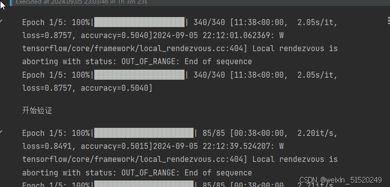
五、训练模型
# 训练模型
from tqdm import tqdm
import tensorflow.keras.backend as K
epochs = 5
lr = 1e-4
history_train_loss = []
history_train_accuracy = []
history_val_loss = []
history_val_accuracy = []
for epoch in range(epochs):
train_total = len(train_ds)
val_total = len(val_ds)
with tqdm(total=train_total, desc=f'Epoch {epoch + 1}/{epochs}', mininterval=1, ncols=100) as pbar:
lr = lr * 0.92
learning_rate = lr
# 更新学习率
# K.set_value(model.optimizer.learning_rate, lr)
for image, label in train_ds:
history = model.train_on_batch(image, label)
train_loss = history[0]
train_accuracy = history[1]
pbar.set_postfix({"loss": "%.4f" % train_loss,
"accuracy": "%.4f" % train_accuracy
}) # 确保获取学习率
pbar.update(1)
history_train_loss.append(train_loss)
history_train_accuracy.append(train_accuracy)
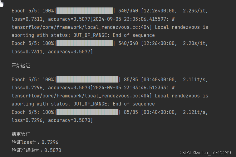
print("开始验证")
with tqdm(total=val_total, desc=f'Epoch {epoch + 1}/{epochs}', mininterval=0.3, ncols=100) as pbar:
for image, label in val_ds:
history = model.test_on_batch(image, label)
val_loss = history[0]
val_accuracy = history[1]
pbar.set_postfix({"loss": "%.4f" % val_loss,
"accuracy": "%.4f" % val_accuracy})
pbar.update(1)
history_val_loss.append(val_loss)
history_val_accuracy.append(val_accuracy)
print('结束验证')
print("验证loss为:%.4f" % val_loss)
print("验证准确率为:%.4f" % val_accuracy)
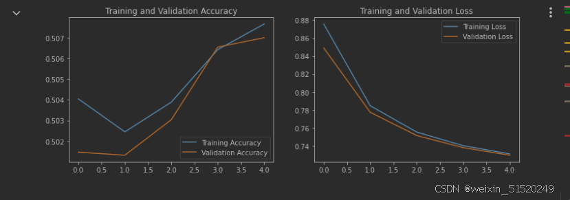
六、模型评估
epochs_range = range(epochs)

plt.figure(figsize=(12, 4))
plt.subplot(1, 2, 1)

plt.plot(epochs_range, history_train_accuracy, label='Training Accuracy')
plt.plot(epochs_range, history_val_accuracy, label='Validation Accuracy')
plt.legend(loc='lower right')
plt.title('Training and Validation Accuracy')

plt.subplot(1, 2, 2)
plt.plot(epochs_range, history_train_loss, label='Training Loss')
plt.plot(epochs_range, history_val_loss, label='Validation Loss')
plt.legend(loc='upper right')
plt.title('Training and Validation Loss')
plt.show()
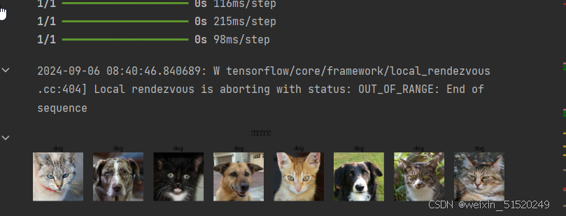
七、预测
import numpy as np

# 采用加载的模型(new_model)来看预测结果
plt.figure(figsize=(18, 3))  # 图形的宽为18高为5
plt.suptitle("预测结果展示")

for images, labels in val_ds.take(1):
    for i in range(8):
        ax = plt.subplot(1,8, i + 1)

        # 显示图片
        plt.imshow(images[i].numpy())

        # 需要给图片增加一个维度
        img_array = tf.expand_dims(images[i], 0)

        # 使用模型预测图片中的人物
        predictions = model.predict(img_array)
        plt.title(class_names[np.argmax(predictions)])

        plt.axis("off")
八、个人总结
在训练模型那一部分
AttributeError                            Traceback (most recent call last)
Cell In[72], line 41
     36     train_loss     = history[0]
     37     train_accuracy = history[1]
     39     pbar.set_postfix({"loss": "%.4f"%train_loss,
     40                       "accuracy":"%.4f"%train_accuracy,
---> 41                       "lr": K.get_value(model.optimizer.lr)})
     42     pbar.update(1)
     43 history_train_loss.append(train_loss)

AttributeError: 'Adam' object has no attribute 'lr'
这里一直报错 查到原因好像因为tensorflow版本不一致和Adam没有lr这个参数 已经改为了learning_rate,但是 我多次尝试 也没有解决。于是就把自动更新学习率那一部分注释掉了
还有一个就是我把epoch设置为了5 服务器内存不足 多人要用 就把epoch改小了。
后续有时间会把这个再给完善一下 或者不使用Adam优化器了。


 1053
1053

 被折叠的 条评论
为什么被折叠?
被折叠的 条评论
为什么被折叠?
 到【灌水乐园】发言


