


GROMACS Tutorial GROMACS 教程
Protein-Ligand Complex 蛋白质-配体复合物
Justin A. Lemkul, Ph.D. 贾斯汀·A·勒姆库尔,博士
Virginia Tech Department of Biochemistry
弗吉尼亚理工大学生物化学系
| This example will guide a new user through the process of setting up a simulation system containing a protein (T4 lysozyme L99A/M102Q) in complex with a ligand. This tutorial focuses specifically on issues related to dealing with the ligand, assuming that the user is familiar with basic GROMACS operations and the contents of a topology. If this is not the case, please refer to a more basic tutorial before attempting this one. This tutorial requires a GROMACS version in the 2018.x series. |
Step One: Prepare the Protein Topology
第一步:准备蛋白质拓扑结构

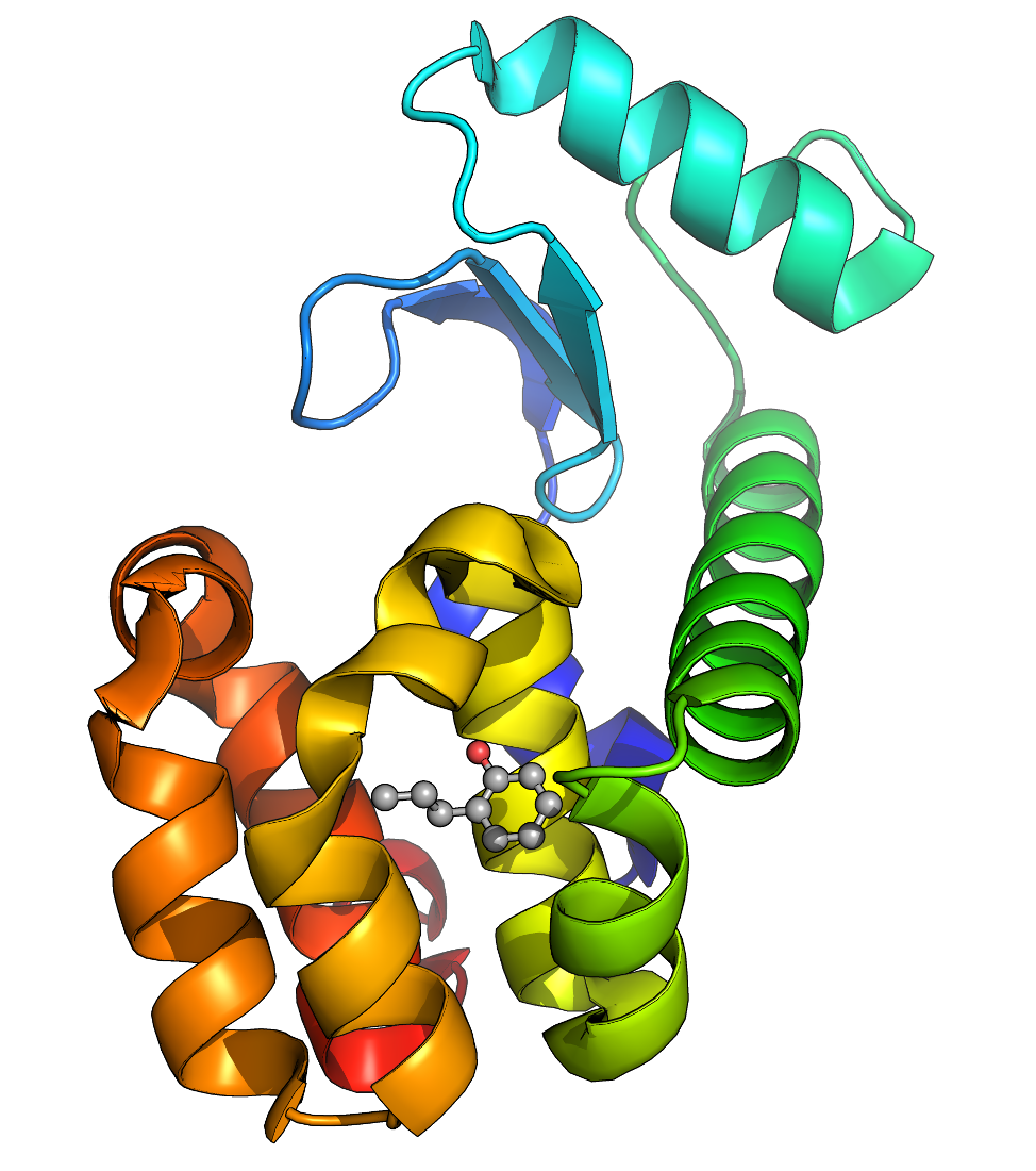
| We must download the protein structure file we will be working with. For this tutorial, we will utilize T4 lysozyme L99A/M102Q (PDB code 3HTB). Go to the RCSB website and download the PDB text for the crystal structure. Once you have downloaded the structure, you can visualize it using a viewing program such as VMD, Chimera, PyMOL, etc. Once you've had a look at the molecule, you are going to want to strip out the crystal waters, PO4, and BME. Note that such a procedure is not universally appropriate (i.e., the case of a bound active site water molecule). For our intentions here, we do not need crystal water or other species, which are just crystallization co-solvents. We will instead focus on the ligand called "JZ4," which is 2-propylphenol. If you want a clean version of the .pdb file to check your work, you can download it here. The problem we now face is that the JZ4 ligand is not a recognized entity in any of the force fields provided with GROMACS, so pdb2gmx will give a fatal error if you were try to pass this file through it. Topologies can only be assembled automatically if an entry for a building block is present in the .rtp (residue topology) file for the force field. Since this is not the case, we will prepare our system topology in two steps:
Since we will be preparing these two topologies separately, we must save the protein and JZ4 ligand into separate coordinate files. Save the JZ4 coordinates like so: grep JZ4 3HTB_clean.pdb > jz4.pdb
Then simply delete the JZ4 lines from 3HTB_clean.pdb. At this point, preparing the protein topology is trivial. The force field we will be using in this tutorial is CHARMM36, obtained from the MacKerell lab website. While there, download the latest CHARMM36 force field tarball and the "cgenff_charmm2gmx.py" conversion script, which we will use later. Download the version of the conversion script that corresponds to your installed Python version (Python 2.x or 3.x). Unarchive the force field tarball in your working directory: tar -zxvf charmm36-jul2022.ff.tgz
There should now be a "charmm36-jul2022.ff" subdirectory in your working directory. Write the topology for the T4 lysozyme with pdb2gmx: gmx pdb2gmx -f 3HTB_clean.pdb -o 3HTB_processed.gro -ter
You will be prompted to make 3 selections.
Select the Force Field:
From current directory:
 1: CHARMM36 all-atom force field (July 2022)
From '/usr/local/gromacs/share/gromacs/top':
 2: AMBER03 protein, nucleic AMBER94 (Duan et al., J. Comp. Chem. 24, 1999-2012, 2003)
 3: AMBER94 force field (Cornell et al., JACS 117, 5179-5197, 1995)
 4: AMBER96 protein, nucleic AMBER94 (Kollman et al., Acc. Chem. Res. 29, 461-469, 1996)
 5: AMBER99 protein, nucleic AMBER94 (Wang et al., J. Comp. Chem. 21, 1049-1074, 2000)
 6: AMBER99SB protein, nucleic AMBER94 (Hornak et al., Proteins 65, 712-725, 2006)
 7: AMBER99SB-ILDN protein, nucleic AMBER94 (Lindorff-Larsen et al., Proteins 78, 1950-58, 2010)
 8: AMBERGS force field (Garcia & Sanbonmatsu, PNAS 99, 2782-2787, 2002)
 9: CHARMM27 all-atom force field (CHARM22 plus CMAP for proteins)
10: GROMOS96 43a1 force field
11: GROMOS96 43a2 force field (improved alkane dihedrals)
12: GROMOS96 45a3 force field (Schuler JCC 2001 22 1205)
13: GROMOS96 53a5 force field (JCC 2004 vol 25 pag 1656)
14: GROMOS96 53a6 force field (JCC 2004 vol 25 pag 1656)
15: GROMOS96 54a7 force field (Eur. Biophys. J. (2011), 40,, 843-856, DOI: 10.1007/s00249-011-0700-9)
16: OPLS-AA/L all-atom force field (2001 aminoacid dihedrals)
For this tutorial, choose the CHARMM36 force field (option 1), listed first under "From current directory" in the list. Choose the default water model (CHARMM-modified TIP3P) and then choose "NH3+" and "COO-" for the termini. This interactive selection is necessary due to the N-terminal residue being methionine (MET), which causes pdb2gmx to choose an incompatible terminus type that is intended for carbohydrates. You must select the protein-specific termini, otherwise you will get a fatal error about non-matching atom names. |
Step Two: Prepare the Ligand Topology
第二步:准备配体拓扑
| We must now deal with the ligand. But how does one come up with parameters for some species that the force field does not automatically recognize? Proper treatment of ligands is one of the most challenging tasks in molecular simulation. Force field authors spend years of their lives deriving self-consistent force fields, and it is no small task to introduce a new species into this framework. Force field parameters for any new species must be derived and validated in a manner that is consistent with the original force field. For the OPLS, AMBER, and CHARMM force fields, this derivation often takes the form of various quantum mechanical calculations. The primary literature for these force fields describes the required procedure. For GROMOS force fields, parameterization methodology is less clear, relying on empirical fitting of condensed-phase behavior. That is, some initial charges and Lennard-Jones parameters are calculated for each atom type, evaluated for their accuracy, and refined. While the end result is very satisfactory, i.e. fluids resemble their real-world counterparts, the derivation process can be laborious and frustrating. For this reason, automated tools are greatly preferred. For each force field, there are methodologies or software programs that purport to give parameters compatible with various force fields. Not all of them are equally accurate. For a few examples, refer to the following table:
Add Hydrogen Atoms to JZ4 | |||||||||||||||||||||||||||||||||
Step Three: Defining the Unit Cell & Adding Solvent
第三步:定义晶胞并添加溶剂

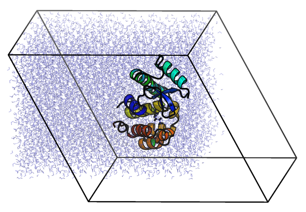
| At this point, the workflow is just like any other MD simulation. We will define the unit cell and fill it with water. gmx editconf -f complex.gro -o newbox.gro -bt dodecahedron -d 1.0
gmx solvate -cp newbox.gro -cs spc216.gro -p topol.top -o solv.gro
Upon visualizing
GROMACS programs always use the most numerically efficient representation of the coordinates, one that has everything re-wrapped into a triclinic unit cell. The physical calculations that mdrun performs can be carried out equivalently with different coordinate wrapping, so the most efficient is preferred. The desired unit cell shape can be recovered later, following the generation of a .tpr file. |
Step Four: Adding Ions 第四步:添加离子

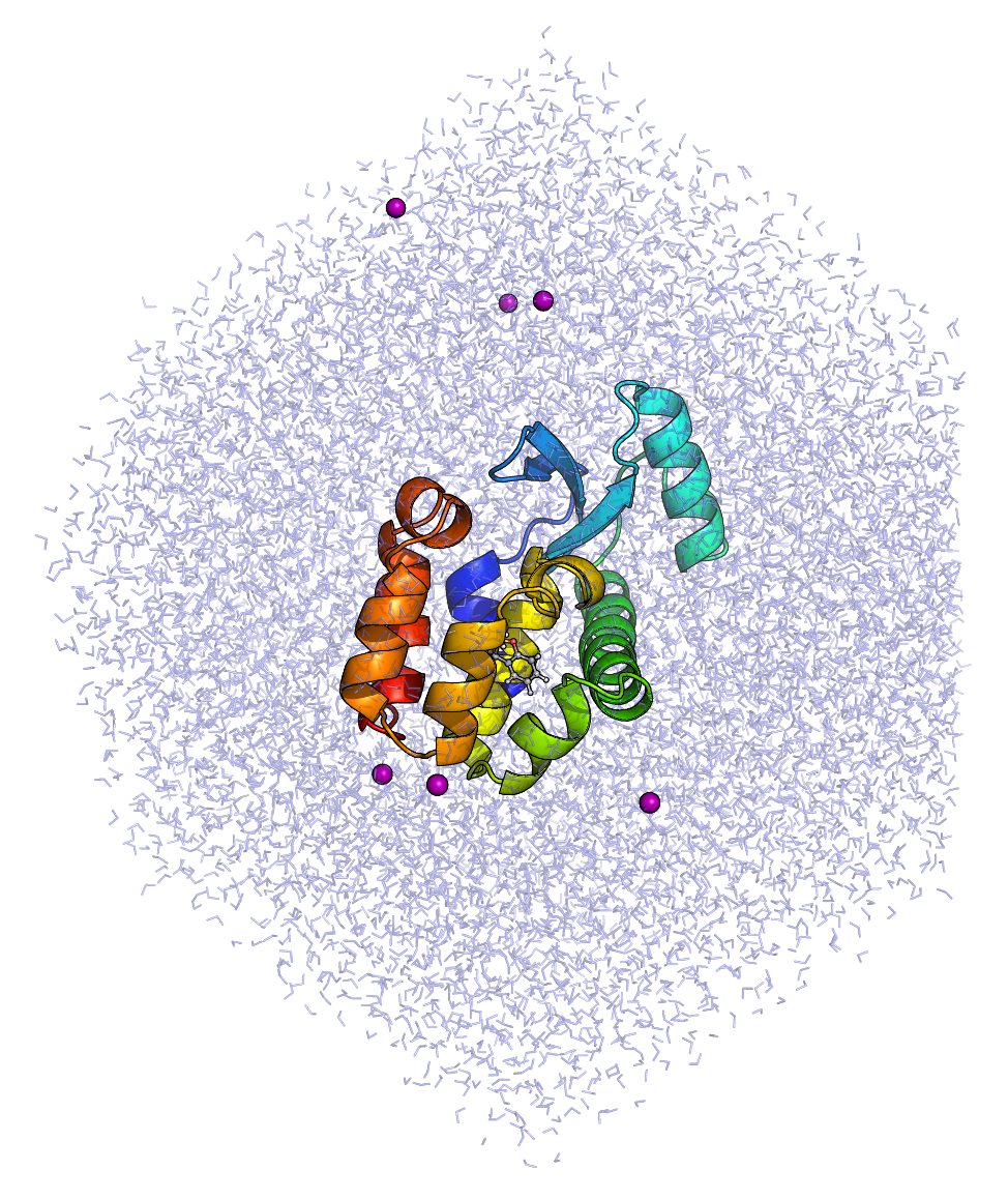
| We now have a solvated system that contains a charged protein. The output of pdb2gmx told us that the protein has a net charge of +6e (based on its amino acid composition). If you missed this information in the pdb2gmx output, look at the last line of your Use grompp to assemble a .tpr file, using any .mdp file. I use an .mdp file for running energy minimization, since they require the fewest parameters and are thus the easiest to maintain. For example, this one. gmx grompp -f ions.mdp -c solv.gro -p topol.top -o ions.tpr
We now pass our .tpr file to genion: gmx genion -s ions.tpr -o solv_ions.gro -p topol.top -pname NA -nname CL -neutral
The names of the ions specified with -pname and -nname were force field-specific in previous versions of GROMACS, but were standardized in version 4.5. The specified atom names are always the elemental symbol in all capital letters, along with the Your [ molecules ]
; Compound #mols
Protein_chain_A 1
JZ4 1
SOL 10228
CL 6
|
Step Five: Energy Minimization
第五步:能量最小化

| Now that the system is assembled, create the binary input using grompp using this input parameter file: gmx grompp -f em.mdp -c solv_ions.gro -p topol.top -o em.tpr
Make sure you have been updating your topol.top file when running genbox and genion, or else you will get lots of nasty error messages ("number of coordinates in coordinate file does not match topology," etc). We are now ready to invoke mdrun to carry out the EM: gmx mdrun -v -deffnm em
For me, the system converged relatively quickly: Steepest Descents converged to Fmax < 1000 in 143 steps
Potential Energy = -4.9014547e+05
Maximum force = 8.7411469e+02 on atom 27
Norm of force = 5.6676244e+01
As in the lysozyme tutorial, it is possible to monitor various components of the potential energy using the energy module. I will not illustrate these principles here. Have fun. Now that our system is at an energy minimum, we can begin real dynamics. |
Step Six: Equilibration 第六步:平衡

| Equilibrating our protein-ligand complex will be much like equilibrating any other system containing a protein in water. There are a few special considerations, in this case:
Restraining the Ligand 约束配体To restrain the ligand, we will need to generate a position restraint topology for it. First, create an index group for JZ4 that contains only its non-hydrogen atoms: gmx make_ndx -f jz4.gro -o index_jz4.ndx
...
> 0 & ! a H*
> q
Then, execute the genrestr module and select this newly created index group (which will be group 3 in the index_jz4.ndx file): gmx genrestr -f jz4.gro -n index_jz4.ndx -o posre_jz4.itp -fc 1000 1000 1000
Now, we need to include this information in our topology. We can do this in several ways, depending upon the conditions we wish to use. If we simply want to restrain the ligand whenever the protein is also restrained, add the following lines to your topology in the location indicated: ; Include Position restraint file
#ifdef POSRES
#include "posre.itp"
#endif
; Include ligand topology
#include "jz4.itp"
; Ligand position restraints
#ifdef POSRES
#include "posre_jz4.itp"
#endif
; Include water topology
#include "./charmm36-jul2022.ff/tip3p.itp"
Location matters! You must put the call for posre_jz4.itp in the topology as indicated. The parameters within jz4.itp define a If you want a bit more control during equilibration, i.e. restraining the protein and ligand independently, you could instead control the inclusion of the ligand position restraint file in a different #ifdef block, like so: ; Include Position restraint file
#ifdef POSRES
#include "posre.itp"
#endif
; Include ligand topology
#include "jz4.itp"
; Ligand position restraints
#ifdef POSRES_LIG
#include "posre_jz4.itp"
#endif
; Include water topology
#include "./charmm36-jul2022.ff/tip3p.itp"
In the latter case, to restrain both the protein and the ligand, we would need to specify Thermostats 恒温器Proper control of temperature coupling is a sensitive issue. Coupling every moleculetype to its own thermostatting group is a bad idea. For instance, if you do the following: tc-grps = Protein JZ4 SOL CL
Your system will probably blow up, since the temperature coupling algorithms are not stable enough to control the fluctuations in kinetic energy that groups with a few atoms (i.e., JZ4 and CL) will produce. Do not couple every single species in your system separately. The typical approach is to set gmx make_ndx -f em.gro -o index.ndx
...
0 System : 33506 atoms
1 Protein : 2614 atoms
2 Protein-H : 1301 atoms
3 C-alpha : 163 atoms
4 Backbone : 489 atoms
5 MainChain : 651 atoms
6 MainChain+Cb : 803 atoms
7 MainChain+H : 813 atoms
8 SideChain : 1801 atoms
9 SideChain-H : 650 atoms
10 Prot-Masses : 2614 atoms
11 non-Protein : 30892 atoms
12 Other : 22 atoms
13 JZ4 : 22 atoms
14 CL : 6 atoms
15 Water : 30864 atoms
16 SOL : 30864 atoms
17 non-Water : 2642 atoms
18 Ion : 6 atoms
19 JZ4 : 22 atoms
20 CL : 6 atoms
21 Water_and_ions : 30870 atoms
Merge the "Protein" and "JZ4" groups with the following, where ">" indicates the make_ndx prompt: > 1 | 13
> q
We can now set Proceed with NVT equilibration using this .mdp file. gmx grompp -f nvt.mdp -c em.gro -r em.gro -p topol.top -n index.ndx -o nvt.tpr
gmx mdrun -deffnm nvt |
Step Seven: Equilibration, Part 2
第七步:平衡,第二部分
| Once the NVT simulation is complete, proceed to NPT with this .mdp file: gmx grompp -f npt.mdp -c nvt.gro -t nvt.cpt -r nvt.gro -p topol.top -n index.ndx -o npt.tpr
gmx mdrun -deffnm npt |
Step Eight: Production MD
步骤八:生产 MD

| Upon completion of the two equilibration phases, the system is now well-equilibrated at the desired temperature and pressure. We are now ready to release the position restraints and run production MD for data collection. The process is just like we have seen before, as we will make use of the checkpoint file (which in this case now contains preserve pressure coupling information) to grompp. We will run a 10-ns MD simulation, the script for which can be found here. gmx grompp -f md.mdp -c npt.gro -t npt.cpt -p topol.top -n index.ndx -o md_0_10.tpr
gmx mdrun -deffnm md_0_10 |
Step Nine: Analysis 步骤九:分析

Recentering and Rewrapping Coordinates |
Summary 摘要
| You have now conducted a molecular dynamics simulation of a protein-ligand complex with GROMACS. This tutorial should not be viewed as comprehensive. There are many more types of simulations that one can conduct with GROMACS (free energy calculations, non-equilibrium MD, and normal modes analysis, just to name a few). You should also review the literature and the GROMACS manual for adjustments to the .mdp files provided here for efficiency and accuracy purposes. If you have suggestions for improving this tutorial, if you notice a mistake, or if anything is otherwise unclear, please feel free to email me. Please note: this is not an invitation to email me for GROMACS problems. I do not advertise myself as a private tutor or personal help service. That's what the GROMACS User Forum is for. I may help you there, but only in the context of providing service to the community as a whole, not just the end user. Happy simulating! 模拟愉快! |


 8138
8138

 被折叠的 条评论
为什么被折叠?
被折叠的 条评论
为什么被折叠?
 到【灌水乐园】发言


