1.Keras实现简单线性回归和简单非线性问题

---

前言

笔者也是最近开始学习keras这个深度学习的高级API，它的方便和强大想必不用再多说。正如它文档写的那样：“你恰好发现了keras”。

---

提示：以下是本篇文章正文内容，下面案例可供参考

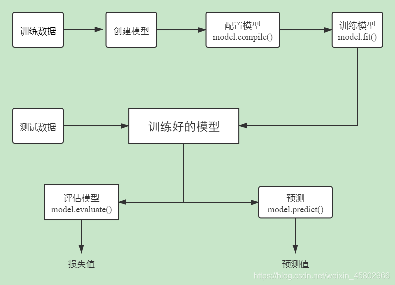
一、keras的工作流程

Keras提供了简明易上手的工作流程，以模型为中心，构建模型，编译模型，使用训练数据训练模型，评估模型。

二、案例

1、实现一个一元一次的线性回归

"""
导入所有需要的库
Sequential 用于堆叠神经网络的序列
Dense 全连接层
Activation 激活层
numpy 强大的计算库
matplotlib.pyplot 绘图工具
"""
import keras
from keras.models import Sequential
from keras.layers import Dense, Activation
import numpy as np
import matplotlib.pyplot as plt


# 1、准备数据
def get_dates(counts):
    Xs = np.random.rand(counts)   # np.random.rand() 通过本函数可以返回一个或一组服从"0-1"均匀分布的随机样本值
    Xs = np.sort(Xs)  # 排序
    # 随便构造一个线性关系(一元一次函数 1.2 * x + 0.5)
    Ys = np.array([(1.2 * x + (0.5 - np.random.rand()) / 5 + 0.5) for x in Xs])
    return Xs, Ys


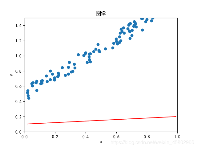
# 2、画出初始散点图和预测图像
ans = 100
xs, ys = get_dates(ans)
plt.rcParams['font.sans-serif'] = ['simhei']  # 防止中文乱码
plt.rcParams['axes.unicode_minus'] = False  # 防止负号乱码
plt.title('图像')
plt.xlabel('x')
plt.ylabel('y')
plt.xlim(0, 1)  # 限制x轴的显示范围
plt.ylim(0, 1.5)  # 限制y轴的显示范围
plt.scatter(xs, ys)  # 绘制散点图

# 预测函数的初始参数值
w = 0.1
b = 0.1
y_pre = w * xs + b
plt.plot(xs, y_pre, c='r')  # 绘制预测函数的直线
# 当然结果是大相径庭
plt.show()

# 3、使用Keras
# 3.1、构建模型
model = Sequential()  # 建立序贯模型
model.add(Dense(units=1, input_dim=1))  # units=当前层神经元数量, input_dim=输入数据的维度, activation=激活函数的类型(激活函数是解决非线性问题所以在这里不需要设置)

# 3.2、编译模型
# optimizer=优化器(adam(实践表明，Adam 比其他适应性学习方法效果要好。)), loss=损失函数(这里我们用均方误差), metrics=评估标准(准确度)
model.compile(optimizer='adam', loss='mean_squared_error', metrics=['accuracy'])

# 3.3、训练模型
model.fit(xs, ys, epochs=5000, batch_size=20)  # epochs=回合数, batch_size=批数量
# 这里就是我总训练次数5000次， 每次训练数据一批20次

# 3.4 预测模型
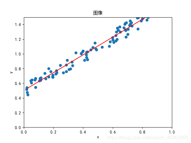
y_pre = model.predict(xs)

# 绘制图像进行对比
plt.rcParams['font.sans-serif'] = ['simhei']  # 防止中文乱码
plt.rcParams['axes.unicode_minus'] = False  # 防止负号乱码
plt.title('图像')
plt.xlabel('x')
plt.ylabel('y')
plt.xlim(0, 1)  # 限制x轴的显示范围
plt.ylim(0, 1.5)  # 限制y轴的显示范围
plt.scatter(xs, ys)  # 绘制散点图
plt.plot(xs, y_pre, c='r')  # 再次绘制预测直线
plt.show()

# 比方预测x == 150
# y = 1.2 * 150 + 0.5
print(model.predict([150]))  # 结果基本吻合

运行结果

---

2、实现一个简单的非线性问题

"""
导入所有需要的库
Sequential 用于堆叠神经网络的序列
Dense 全连接层
Activation 激活层
numpy 强大的计算库
matplotlib.pyplot 绘图工具
"""
import keras
from keras.models import Sequential
from keras.layers import Dense, Activation
import numpy as np
import matplotlib.pyplot as plt


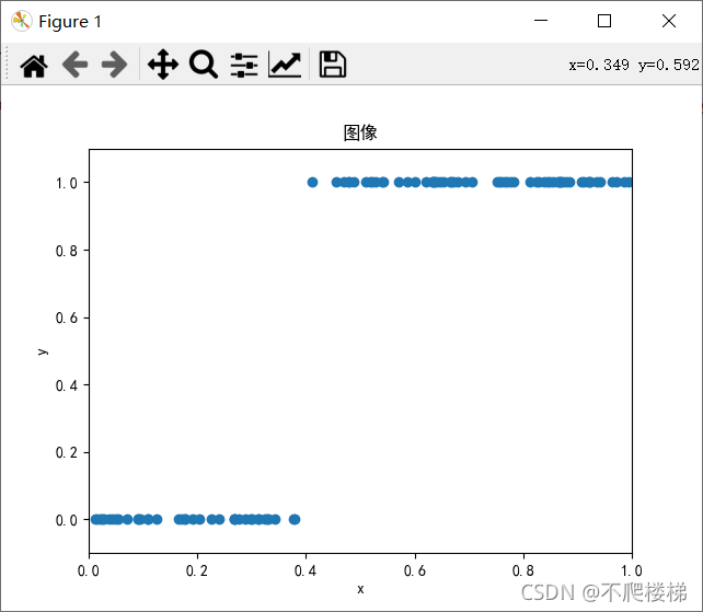
# 准备数据，最后结果无非就两种情况[0, 1]
def get_data(ans):
    X = np.sort(np.random.rand(ans))
    Y = []

    for x in X:
        y = 1.2 * x + (0.5 - np.random.rand()) / 5 + 0.5
        if y > 1:
            Y.append(1)
        else:
            Y.append(0)

    return X, Y


m = 100
X, Y = get_data(m)
plt.rcParams['font.sans-serif'] = ['simhei']  # 防止中文乱码
plt.rcParams['axes.unicode_minus'] = False  # 防止负号乱码
plt.title('图像')
plt.xlabel('x')
plt.ylabel('y')
plt.xlim(0, 1)  # 限制x轴的显示范围
plt.ylim(-0.1, 1.1)  # 限制y轴的显示范围
plt.scatter(X, Y)
plt.show()

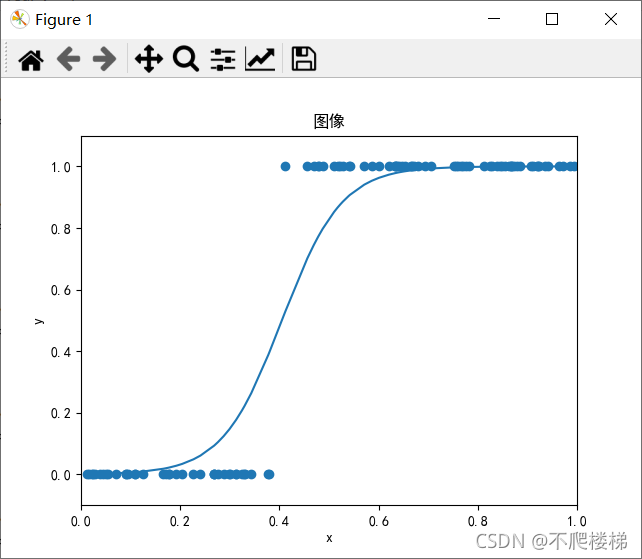
model = Sequential()
# 因为结果无非就是0或者1，相当于实现一个二分类，所以激活函数用'sigmoid'
model.add(Dense(units=1, activation='sigmoid', input_dim=1))

# 损失函数用'binary_crossentropy'(二进制交叉熵,多用于二分类)
model.compile(loss='binary_crossentropy', optimizer='adam', metrics=['accuracy'])
model.fit(X, Y, epochs=5000, batch_size=16)
pres = model.predict(X)

plt.rcParams['font.sans-serif'] = ['simhei']  # 防止中文乱码
plt.rcParams['axes.unicode_minus'] = False  # 防止负号乱码
plt.title('图像')
plt.xlabel('x')
plt.ylabel('y')
plt.xlim(0, 1)  # 限制x轴的显示范围
plt.ylim(-0.1, 1.1)  # 限制y轴的显示范围
plt.scatter(X, Y)
plt.plot(X, pres)
plt.show()

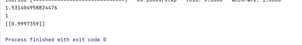
# 测试
# 以0.9为例
real_y = 1.2 * 0.9 + (0.5 - np.random.rand()) / 5 + 0.5  # 这个是真实的结果
print(real_y)
# 如果结果 > 1 那么就输出1否则输出0
if real_y > 1:
    print(1)
else:
    print(0)
# 预测值接近于1
print(model.predict([0.9]))

运行结果

总结

借鉴了《零基础入门Python深度学习》这本书，实现了一个简单了一元一次线性模型和一个简单的非线性问题。其中还有很多的知识在等着我去继续学习！😀