


【1】引言
前序学习进程中,对模拟退火算法的实际计算过程进行了仔细分析,对算法的本质有了更为深入的理解,相关文章链接为:
python学智能算法(二)|模拟退火算法:进阶分析-优快云博客
在此基础上,本次文章将对一些示例进行探索。
【2】原理回忆
前序文章中,已经分析获得模拟退火算法中各个参数的意义:
- 实际上,初始温度和最低温度都不参与计算,它们只是辅助决定要计算多少次。
- 真正实施的计算过程,是在初始温度时,从初始解开始,对初始解周围的区域进行搜索。当搜索次数达到预设数量时,温度降低。
- 在这个过程中,温度不参与计算,只是相当于一个条件,只要温度还没有到最低,搜索过程就要进行。
- 类似于温度就是一个跑道,计算过程就是粒子在奔跑。只要这个跑道还有直径,里面的粒子就要绕着跑道运动,且每个直径的跑道上,粒子运动的圈数相同。
实际运算过程中:
- 当前解和当前能量图可能会向着横坐标减小的方向变化,这表明退火过程中在不断搜索;
- 最优解和最优能量图有时候不会变化,这是因为当前解在搜索过程中,不能发现更好的最优能量,所以最优解和最优能量不会更新;
- 当前解和最优能量图中,最优能量会沿着坐标轴减小到方向往水平方向延展,这就是因为当前解在搜索过程中,不能发现更好的最优能量,所以最优能量不会更新,只会保持之前取到的值。
在前述学习进程中,使用代码以动态图的形式展示了模拟退火算法计算过程中的数据变化,代码为:
import numpy as np
import matplotlib.pyplot as plt
import matplotlib.animation as animation

# 设置 matplotlib 支持中文
plt.rcParams['font.family'] = 'SimHei'
# 解决负号显示问题
plt.rcParams['axes.unicode_minus'] = False

# 定义目标函数,这里是 f(x) = x^2
def objective_function(x):
    return x ** 2

# 初始化参数
# 初始解
initial_solution = np.random.uniform(-10, 10)
# 初始温度
initial_temperature = 100
# 终止温度
final_temperature = 0.01
# 温度衰减系数
alpha = 0.95
# 每个温度下的迭代次数
num_iterations_per_temp = 5

# 模拟退火算法
def simulated_annealing(initial_solution, initial_temperature, final_temperature, alpha, num_iterations_per_temp):
    # 当前解
    current_solution = initial_solution
    # 当前解的目标函数值
    current_energy = objective_function(current_solution)
    # 最优解
    best_solution = current_solution
    # 最优解的目标函数值
    best_energy = current_energy
    # 当前温度
    temperature = initial_temperature

    # 用于记录每一步的最优目标函数值
    energy_history = [best_energy]
    current_solution_history = [current_solution]
    current_energy_history = [current_energy]
    best_energy_history = [best_energy]
    best_solution_history =[best_solution]

    while temperature > final_temperature:
        for _ in range(num_iterations_per_temp):
            # 在当前解的邻域内生成新解
            new_solution = current_solution + np.random.uniform(-0.1, 0.1)
            # 计算新解的目标函数值
            new_energy = objective_function(new_solution)
            # 计算能量差
            delta_energy = new_energy - current_energy

            # 如果新解更优,直接接受
            if delta_energy < 0:
                current_solution = new_solution
                current_energy = new_energy
                # 更新最优解
                if new_energy < best_energy:
                    best_solution = new_solution
                    best_energy = new_energy
            # 如果新解更差,以一定概率接受
            else:
                acceptance_probability = np.exp(-delta_energy / temperature)
                if np.random.rand() < acceptance_probability:
                    current_solution = new_solution
                    current_energy = new_energy

            # 记录当前最优目标函数值
            energy_history.append(best_energy)
            # 更新当前解和能量的历史记录
            current_solution_history.append(current_solution)
            current_energy_history.append(current_energy)
            best_energy_history.append(best_energy)
            best_solution_history.append(best_solution)

        # 降低温度
        temperature *= alpha

    return best_solution, best_energy, energy_history, current_solution_history, current_energy_history, best_energy_history, best_solution_history

# 运行模拟退火算法
best_solution, best_energy, energy_history, current_solution_history, current_energy_history, best_energy_history, best_solution_history= simulated_annealing(
    initial_solution, initial_temperature, final_temperature, alpha, num_iterations_per_temp)

print("最优解:", best_solution)
print("最优值:", best_energy)
print('energy_history=', energy_history)

fig, ax = plt.subplots()  # 定义要画图
# 设置坐标轴范围
#ax.set_xlim(min(current_solution_history), max(current_solution_history))
#ax.set_ylim(min(current_energy_history), max(current_energy_history))
ax.set_xlim(-10,10)
ax.set_ylim(0,100)
# 定义散点图对象
scatter1 = ax.scatter([], [], c='b', label='当前解与当前能量关系')
scatter2 = ax.scatter([], [], c='g', marker="^",label='最优解与最优能量关系')
# 定义折线图对象来表示 best_energy 的变化
line, = ax.plot([], [], 'r-', label='当前解与最优能量关系')

num_frames = len(energy_history)
x = np.linspace(-10, 10, 400)
y = objective_function(x)
plt.plot(x, y, label='目标函数')
def update(frame):
    x = current_solution_history[:frame + 1]
    y = current_energy_history[:frame + 1]
    # 更新散点图的数据
    scatter1.set_offsets(np.c_[x, y])

    # 更新折线图的数据,这里使用迭代步数作为 x 轴,best_energy 作为 y 轴
    line_x = current_solution_history[:frame + 1]
    line_y = best_energy_history[:frame + 1]
    line.set_data(line_x, line_y)

    scatter_x=best_solution_history[:frame + 1]
    scatter_y =best_energy_history[:frame + 1]
    scatter2.set_offsets(np.c_[scatter_x, scatter_y])

    return scatter1, line,scatter2

ani = animation.FuncAnimation(fig, update, repeat=True,
                              frames=num_frames, interval=50)  # 调用animation.FuncAnimation()函数画图
plt.legend()

ani.save('mnthsf.gif') #保存动画
plt.show()
上述代码运行后,会出现动画,展示详细的计算过程。
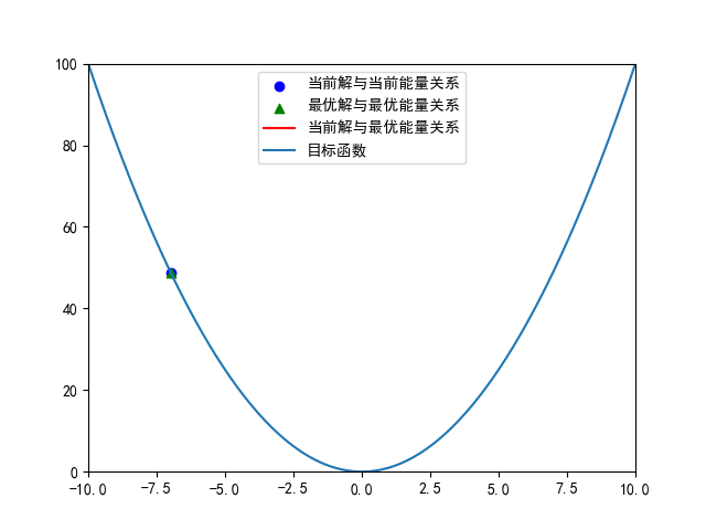
图1 模拟退火算法动画显示
有时候为了更清晰展示各个计算过程的变化,需要使用多子图来显示。于是对上述代码稍加修改,变成下述形式,代码运行后不再显示动画,而是分成两个子图显示参数的变化情况:
import numpy as np
import matplotlib.pyplot as plt
import matplotlib.animation as animation

# 设置 matplotlib 支持中文
plt.rcParams['font.family'] = 'SimHei'
# 解决负号显示问题
plt.rcParams['axes.unicode_minus'] = False

# 定义目标函数,这里是 f(x) = x^2
def objective_function(x):
    return x ** 2

# 初始化参数
# 初始解
initial_solution = np.random.uniform(-10, 10)
# 初始温度
initial_temperature = 100
# 终止温度
final_temperature = 0.01
# 温度衰减系数
alpha = 0.95
# 每个温度下的迭代次数
num_iterations_per_temp = 5

# 模拟退火算法
def simulated_annealing(initial_solution, initial_temperature, final_temperature, alpha, num_iterations_per_temp):
    # 当前解
    current_solution = initial_solution
    # 当前解的目标函数值
    current_energy = objective_function(current_solution)
    # 最优解
    best_solution = current_solution
    # 最优解的目标函数值
    best_energy = current_energy
    # 当前温度
    temperature = initial_temperature

    # 用于记录每一步的最优目标函数值
    energy_history = [best_energy]
    current_solution_history = [current_solution]
    current_energy_history = [current_energy]
    best_energy_history = [best_energy]
    best_solution_history =[best_solution]

    while temperature > final_temperature:
        for _ in range(num_iterations_per_temp):
            # 在当前解的邻域内生成新解
            new_solution = current_solution + np.random.uniform(-0.1, 0.1)
            # 计算新解的目标函数值
            new_energy = objective_function(new_solution)
            # 计算能量差
            delta_energy = new_energy - current_energy

            # 如果新解更优,直接接受
            if delta_energy < 0:
                current_solution = new_solution
                current_energy = new_energy
                # 更新最优解
                if new_energy < best_energy:
                    best_solution = new_solution
                    best_energy = new_energy
            # 如果新解更差,以一定概率接受
            else:
                acceptance_probability = np.exp(-delta_energy / temperature)
                if np.random.rand() < acceptance_probability:
                    current_solution = new_solution
                    current_energy = new_energy

            # 记录当前最优目标函数值
            energy_history.append(best_energy)
            # 更新当前解和能量的历史记录
            current_solution_history.append(current_solution)
            current_energy_history.append(current_energy)
            best_energy_history.append(best_energy)
            best_solution_history.append(best_solution)

        # 降低温度
        temperature *= alpha

    return best_solution, best_energy, energy_history, current_solution_history, current_energy_history, best_energy_history, best_solution_history

# 运行模拟退火算法
best_solution, best_energy, energy_history, current_solution_history, current_energy_history, best_energy_history, best_solution_history= simulated_annealing(
    initial_solution, initial_temperature, final_temperature, alpha, num_iterations_per_temp)

print("最优解:", best_solution)
print("最优值:", best_energy)
print('energy_history=', energy_history)

# 绘制图形
plt.figure(figsize=(12, 5))
#fig, ax = plt.subplots()  # 定义要画图
# 设置坐标轴范围
#ax.set_xlim(min(current_solution_history), max(current_solution_history))
#ax.set_ylim(min(current_energy_history), max(current_energy_history))
#ax.set_xlim(-10,10)
#ax.set_ylim(0,100)
# 定义散点图对象
#scatter1 = ax.scatter([], [], c='b', label='当前解与当前能量关系')
#scatter2 = ax.scatter([], [], c='g', marker="^",label='最优解与最优能量关系')
# 定义折线图对象来表示 best_energy 的变化
#line, = ax.plot([], [], 'r-', label='当前解与最优能量关系')
plt.subplot(1, 2, 1)
plt.suptitle('模拟退火算法',y=0.95) #设置图像名称
num_frames = len(energy_history)
x = np.linspace(-10, 10, 400)
y = objective_function(x)
plt.plot(x, y, label='目标函数')
frame = len(energy_history)
x1 = current_solution_history[:frame + 1]
y1 = current_energy_history[:frame + 1]
    # 更新散点图的数据
plt.scatter(x1,y1, c='b', label='当前解与当前能量关系')
plt.scatter(best_solution, best_energy,c='r',marker="^", label='最佳能量')
plt.legend()
plt.subplot(1, 2, 2)
line_x = current_solution_history[:frame + 1]
line_y = best_energy_history[:frame + 1]
plt.plot(line_x, line_y,c='r', label='当前解与最优能量关系')
scatter_x=best_solution_history[:frame + 1]
scatter_y =best_energy_history[:frame + 1]
plt.scatter(scatter_x,scatter_y, c='g', marker="^",label='最优解与最优能量关系')
plt.legend()

plt.savefig('mnthsf.png')
plt.show()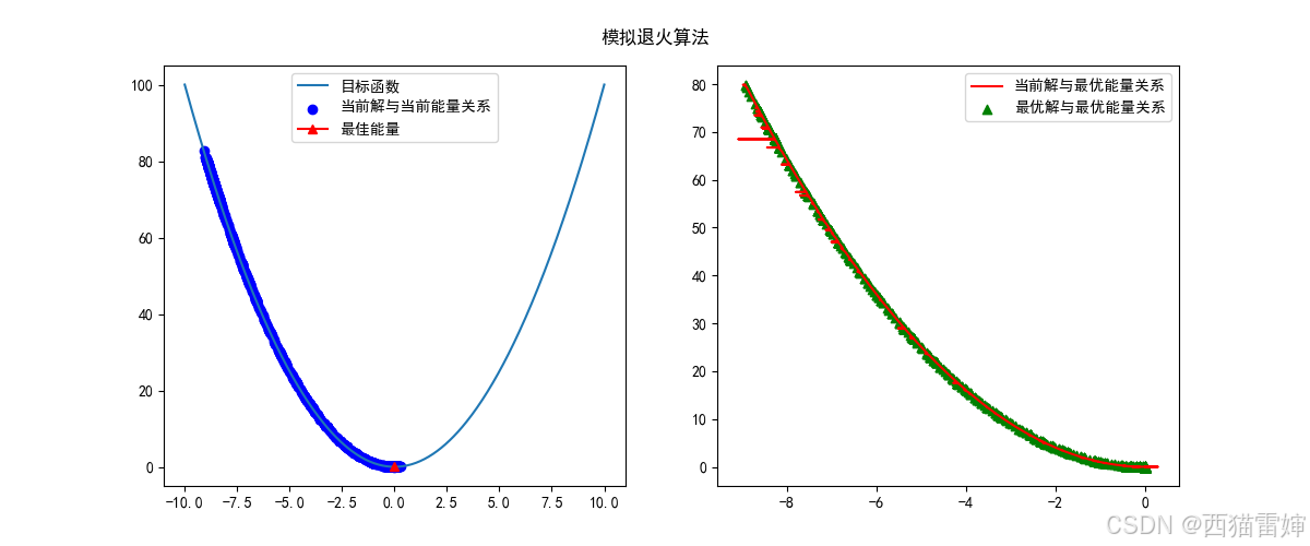
图2 模拟退火算法多图显示
动画和多图都是展示模拟退火算法运行原理和数据处理过程的工具。
也有时候将上述两种显示方式结合,也就是用并排的动画来显示模拟退火算法的变化过程:
import numpy as np
import matplotlib.pyplot as plt
import matplotlib.animation as animation

# 设置 matplotlib 支持中文
plt.rcParams['font.family'] = 'SimHei'
# 解决负号显示问题
plt.rcParams['axes.unicode_minus'] = False


# 定义目标函数,这里是 f(x) = x^2
def objective_function(x):
    return x ** 2


# 初始化参数
# 初始解
initial_solution = np.random.uniform(-10, 10)
# 初始温度
initial_temperature = 100
# 终止温度
final_temperature = 0.01
# 温度衰减系数
alpha = 0.95
# 每个温度下的迭代次数
num_iterations_per_temp = 5


# 模拟退火算法
def simulated_annealing(initial_solution, initial_temperature, final_temperature, alpha, num_iterations_per_temp):
    # 当前解
    current_solution = initial_solution
    # 当前解的目标函数值
    current_energy = objective_function(current_solution)
    # 最优解
    best_solution = current_solution
    # 最优解的目标函数值
    best_energy = current_energy
    # 当前温度
    temperature = initial_temperature

    # 用于记录每一步的最优目标函数值
    energy_history = [best_energy]
    current_solution_history = [current_solution]
    current_energy_history = [current_energy]
    best_energy_history = [best_energy]
    best_solution_history = [best_solution]

    while temperature > final_temperature:
        for _ in range(num_iterations_per_temp):
            # 在当前解的邻域内生成新解
            new_solution = current_solution + np.random.uniform(-0.1, 0.1)
            # 计算新解的目标函数值
            new_energy = objective_function(new_solution)
            # 计算能量差
            delta_energy = new_energy - current_energy

            # 如果新解更优,直接接受
            if delta_energy < 0:
                current_solution = new_solution
                current_energy = new_energy
                # 更新最优解
                if new_energy < best_energy:
                    best_solution = new_solution
                    best_energy = new_energy
            # 如果新解更差,以一定概率接受
            else:
                acceptance_probability = np.exp(-delta_energy / temperature)
                if np.random.rand() < acceptance_probability:
                    current_solution = new_solution
                    current_energy = new_energy

            # 记录当前最优目标函数值
            energy_history.append(best_energy)
            # 更新当前解和能量的历史记录
            current_solution_history.append(current_solution)
            current_energy_history.append(current_energy)
            best_energy_history.append(best_energy)
            best_solution_history.append(best_solution)

        # 降低温度
        temperature *= alpha

    return best_solution, best_energy, energy_history, current_solution_history, current_energy_history, best_energy_history, best_solution_history


# 运行模拟退火算法
best_solution, best_energy, energy_history, current_solution_history, current_energy_history, best_energy_history, best_solution_history = simulated_annealing(
    initial_solution, initial_temperature, final_temperature, alpha, num_iterations_per_temp)

print("最优解:", best_solution)
print("最优值:", best_energy)
print('energy_history=', energy_history)

fig, (ax1, ax2) = plt.subplots(1, 2, sharex=True, sharey=True)  # 定义要画图
plt.suptitle('模拟退火算法',y=0.95) #设置图像名称
# 定义散点图对象
scatter1 = ax1.scatter([], [], c='b', label='当前解与当前能量关系')
scatter2 = ax2.scatter([], [], c='g', marker="^", label='最优解与最优能量关系')
# 定义折线图对象来表示 best_energy 的变化
line, = ax2.plot([], [], 'r-', label='当前解与最优能量关系')

num_frames = len(energy_history)
x = np.linspace(-10, 10, 400)
y = objective_function(x)
ax1.plot(x, y, label='目标函数')

# 在每个子图上分别显示图例
ax1.legend()
ax2.legend()

# 标注最佳能量的坐标值
ax1.scatter(best_solution, best_energy, c='r', marker='o', label='最佳能量坐标')
ax1.text(best_solution, best_energy, f'({best_solution:.2f}, {best_energy:.2f})', fontsize=10, color='r')
ax2.scatter(best_solution, best_energy, c='r', marker='o', label='最佳能量坐标')
ax2.text(best_solution, best_energy, f'({best_solution:.2f}, {best_energy:.2f})', fontsize=10, color='r')

def update(frame):
    x = current_solution_history[:frame + 1]
    y = current_energy_history[:frame + 1]
    # 更新散点图的数据
    scatter1.set_offsets(np.c_[x, y])

    # 更新折线图的数据,这里使用迭代步数作为 x 轴,best_energy 作为 y 轴
    line_x = current_solution_history[:frame + 1]
    line_y = best_energy_history[:frame + 1]
    line.set_data(line_x, line_y)

    scatter_x = best_solution_history[:frame + 1]
    scatter_y = best_energy_history[:frame + 1]
    scatter2.set_offsets(np.c_[scatter_x, scatter_y])

    return scatter1, line, scatter2


ani = animation.FuncAnimation(fig, update, repeat=False,
                              frames=num_frames, interval=50)  # 调用 animation.FuncAnimation() 函数画图

ani.save('mnthsf.gif')  # 保存动画
plt.show()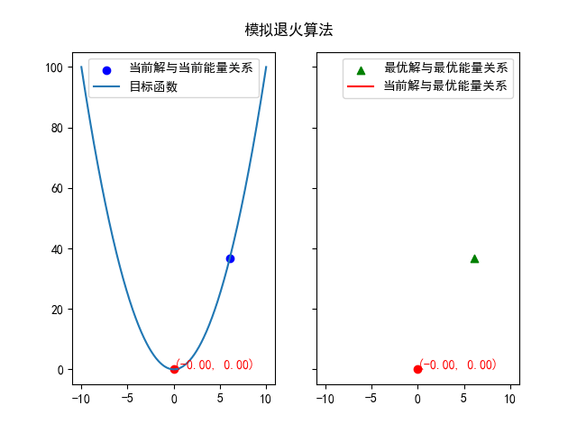
图3 模拟退火算法多动画显示
实际上运算过程中,由于随机性的取初始值,所以同一个程序两次运行的输出图像可能不一样,但最优值往往非常接近。
以上三种表达方式只是可能的三种,大家可以自由选择或者继续创新。
【3】实际应用
在掌握了模拟退火算法实际的运行原理之后,最佳的办法就是通过实践检验。
【3.1】极小值计算
首先测试一个简单的多峰函数,计算最小值,这给出完整代码:
import numpy as np
import matplotlib.pyplot as plt
import matplotlib.animation as animation

# 设置 matplotlib 支持中文
plt.rcParams['font.family'] = 'SimHei'
# 解决负号显示问题
plt.rcParams['axes.unicode_minus'] = False

#定义自变量范围
x_min=0
x_max=5

# 定义目标函数,这里是 f(x) = x^2
def objective_function(x):
    #return x ** 2
    #return np.cos(x) ** 2 + 0.5 * np.cos(2 * x) ** 2
    #return np.sin(x) + np.sin(2 * x) + np.sin(3 * x)
    return x ** 2 * np.sin(5 * x) + 0.1 * x ** 2

# 初始化参数
# 初始解
initial_solution = np.random.uniform(x_min, x_max)
# 初始温度
initial_temperature = 100
# 终止温度
final_temperature = 0.01
# 温度衰减系数
alpha = 0.95
# 每个温度下的迭代次数
num_iterations_per_temp = 5

# 模拟退火算法
def simulated_annealing(initial_solution, initial_temperature, final_temperature, alpha, num_iterations_per_temp):
    # 当前解
    current_solution = initial_solution
    # 当前解的目标函数值
    current_energy = objective_function(current_solution)
    # 最优解
    best_solution = current_solution
    # 最优解的目标函数值
    best_energy = current_energy
    # 当前温度
    temperature = initial_temperature

    # 用于记录每一步的最优目标函数值
    energy_history = [best_energy]
    current_solution_history = [current_solution]
    current_energy_history = [current_energy]
    best_energy_history = [best_energy]
    best_solution_history =[best_solution]

    while temperature > final_temperature:
        for _ in range(num_iterations_per_temp):
            # 在当前解的邻域内生成新解
            new_solution = current_solution + np.random.uniform(-0.1, 0.1)
            # 边界检查,确保新解在自变量范围内
            new_solution = np.clip(new_solution, x_min, x_max)
            # 计算新解的目标函数值
            new_energy = objective_function(new_solution)
            # 计算能量差
            delta_energy = new_energy - current_energy

            # 如果新解更优,直接接受
            if delta_energy < 0:
                current_solution = new_solution
                current_energy = new_energy
                # 更新最优解
                if new_energy < best_energy:
                    best_solution = new_solution
                    best_energy = new_energy
            # 如果新解更差,以一定概率接受
            else:
                acceptance_probability = np.exp(-delta_energy / temperature)
                if np.random.rand() < acceptance_probability:
                    current_solution = new_solution
                    current_energy = new_energy

            # 记录当前最优目标函数值
            energy_history.append(best_energy)
            # 更新当前解和能量的历史记录
            current_solution_history.append(current_solution)
            current_energy_history.append(current_energy)
            best_energy_history.append(best_energy)
            best_solution_history.append(best_solution)

        # 降低温度
        temperature *= alpha

    return best_solution, best_energy, energy_history, current_solution_history, current_energy_history, best_energy_history, best_solution_history

# 运行模拟退火算法
best_solution, best_energy, energy_history, current_solution_history, current_energy_history, best_energy_history, best_solution_history= simulated_annealing(
    initial_solution, initial_temperature, final_temperature, alpha, num_iterations_per_temp)

print("最优解:", best_solution)
print("最优值:", best_energy)
print('energy_history=', energy_history)

# 绘制图形
plt.figure(figsize=(12, 5))
#fig, ax = plt.subplots()  # 定义要画图
# 设置坐标轴范围
#ax.set_xlim(min(current_solution_history), max(current_solution_history))
#ax.set_ylim(min(current_energy_history), max(current_energy_history))
#ax.set_xlim(-10,10)
#ax.set_ylim(0,100)
# 定义散点图对象
#scatter1 = ax.scatter([], [], c='b', label='当前解与当前能量关系')
#scatter2 = ax.scatter([], [], c='g', marker="^",label='最优解与最优能量关系')
# 定义折线图对象来表示 best_energy 的变化
#line, = ax.plot([], [], 'r-', label='当前解与最优能量关系')
plt.subplot(1, 2, 1)
plt.suptitle('模拟退火算法',y=0.95) #设置图像名称
num_frames = len(energy_history)
x = np.linspace(x_min, x_max, 400)
y = objective_function(x)
plt.plot(x, y, label='目标函数')
frame = len(energy_history)
x1 = current_solution_history[:frame + 1]
y1 = current_energy_history[:frame + 1]
    # 更新散点图的数据
plt.scatter(x1,y1, c='b', label='当前解与当前能量关系')
plt.scatter(best_solution, best_energy,c='r',marker="^", label='最佳能量')
# 使用 plt.text() 添加最佳能量坐标标注
plt.text(best_solution-0.5, best_energy+0.5, f'({best_solution:.2f}, {best_energy:.2f})',c='r', fontsize=15)
plt.legend()
plt.subplot(1, 2, 2)
line_x = current_solution_history[:frame + 1]
line_y = best_energy_history[:frame + 1]
plt.plot(line_x, line_y,c='r', label='当前解与最优能量关系')
scatter_x=best_solution_history[:frame + 1]
scatter_y =best_energy_history[:frame + 1]
plt.scatter(scatter_x,scatter_y, c='g', marker="^",label='最优解与最优能量关系')
plt.legend()

plt.savefig('mnthsf.png')
plt.show()
代码运行后获得的图像为:
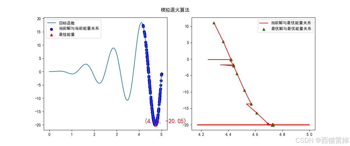
图4 极小值模拟退火算法求解
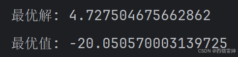
图5 极小值模拟退火算法求解控制台结果
其实如果反复运行代码,每次的结果都可能不一样,甚至有找到其他值的情况。
【3.2】极大值计算
之前都是计算极小值,如果计算极大值,就要更新计算步骤:
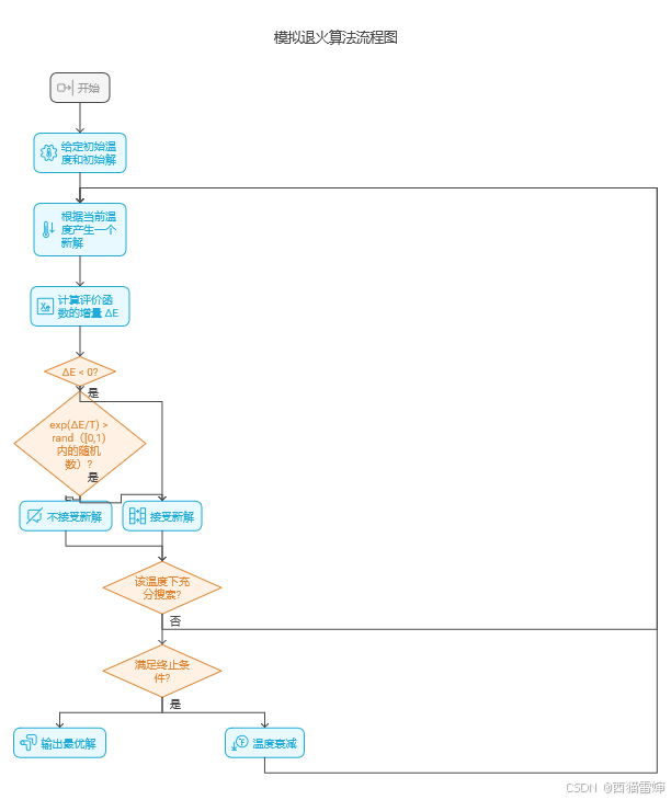
开始:流程的起始点。
给定初始温度和初始解:设定算法开始时的温度值以及问题的一个初始解。初始温度要足够高,以便能够在解空间中充分搜索。
根据当前温度产生一个新解:在当前解的邻域内随机生成一个新的解。
计算评价函数的增量 ΔE:通过计算新解和当前解的评价函数值之差,来衡量新解的优劣。
判断 ΔE 是否小于 0:
如果 ΔE > 0,说明新解比当前解更优,直接接受新解。
如果 ΔE≤ 0,进入下一步判断。
判断 exp (ΔE/T)>rand?:这里涉及到一个概率接受准则。T 是当前温度,rand 是一个 0 到 1 之间的随机数。如果 exp (ΔE/T) 大于 rand,说明以一定概率接受这个较差的新解,这是为了避免算法陷入局部最优解;否则,不接受新解。
判断该温度下充分搜索?:检查在当前温度下是否已经进行了足够多次的搜索。如果没有充分搜索,返回 “根据当前温度产生一个新解” 步骤继续搜索;如果已经充分搜索,则进入下一步。
判断满足终止条件?:检查是否达到了算法的终止条件,如达到最大迭代次数或温度已降至足够低等。如果满足终止条件,输出当前的最优解;如果不满足,则进行温度衰减。
温度衰减:降低当前温度,通常按照一定的降温策略进行,然后返回 “根据当前温度产生一个新解” 步骤,继续搜索过程。
输出最优解:当满足终止条件时,输出找到的最优解,流程结束。
和上一步求极小值使用的函数一样,此处直接修改代码,完整代码为:
import numpy as np
import matplotlib.pyplot as plt
import matplotlib.animation as animation

# 设置 matplotlib 支持中文
plt.rcParams['font.family'] = 'SimHei'
# 解决负号显示问题
plt.rcParams['axes.unicode_minus'] = False

#定义自变量范围
x_min=0
x_max=5

# 定义目标函数,这里是 f(x) = x^2
def objective_function(x):
    #return x ** 2
    #return np.cos(x) ** 2 + 0.5 * np.cos(2 * x) ** 2
    #return np.sin(x) + np.sin(2 * x) + np.sin(3 * x)
    return x ** 2 * np.sin(5 * x) + 0.1 * x ** 2

# 初始化参数
# 初始解
initial_solution = np.random.uniform(x_min, x_max)
# 初始温度
initial_temperature = 100
# 终止温度
final_temperature = 0.01
# 温度衰减系数
alpha = 0.95
# 每个温度下的迭代次数
num_iterations_per_temp = 5

# 模拟退火算法
def simulated_annealing(initial_solution, initial_temperature, final_temperature, alpha, num_iterations_per_temp):
    # 当前解
    current_solution = initial_solution
    # 当前解的目标函数值
    current_energy = objective_function(current_solution)
    # 最优解
    best_solution = current_solution
    # 最优解的目标函数值
    best_energy = current_energy
    # 当前温度
    temperature = initial_temperature

    # 用于记录每一步的最优目标函数值
    energy_history = [best_energy]
    current_solution_history = [current_solution]
    current_energy_history = [current_energy]
    best_energy_history = [best_energy]
    best_solution_history =[best_solution]

    while temperature > final_temperature:
        for _ in range(num_iterations_per_temp):
            # 在当前解的邻域内生成新解
            new_solution = current_solution + np.random.uniform(-0.1, 0.1)
            # 边界检查,确保新解在自变量范围内
            new_solution = np.clip(new_solution, x_min, x_max)
            # 计算新解的目标函数值
            new_energy = objective_function(new_solution)
            # 计算能量差
            delta_energy = new_energy - current_energy

            # 如果新解更优,直接接受
            if delta_energy > 0:
                current_solution = new_solution
                current_energy = new_energy
                # 更新最优解
                if new_energy > best_energy:
                    best_solution = new_solution
                    best_energy = new_energy
            # 如果新解更差,以一定概率接受
            else:
                acceptance_probability = np.exp(delta_energy / temperature)
                if np.random.rand() < acceptance_probability:
                    current_solution = new_solution
                    current_energy = new_energy

            # 记录当前最优目标函数值
            energy_history.append(best_energy)
            # 更新当前解和能量的历史记录
            current_solution_history.append(current_solution)
            current_energy_history.append(current_energy)
            best_energy_history.append(best_energy)
            best_solution_history.append(best_solution)

        # 降低温度
        temperature *= alpha

    return best_solution, best_energy, energy_history, current_solution_history, current_energy_history, best_energy_history, best_solution_history

# 运行模拟退火算法
best_solution, best_energy, energy_history, current_solution_history, current_energy_history, best_energy_history, best_solution_history= simulated_annealing(
    initial_solution, initial_temperature, final_temperature, alpha, num_iterations_per_temp)

print("最优解:", best_solution)
print("最优值:", best_energy)
print('energy_history=', energy_history)

# 绘制图形
plt.figure(figsize=(12, 5))
#fig, ax = plt.subplots()  # 定义要画图
# 设置坐标轴范围
#ax.set_xlim(min(current_solution_history), max(current_solution_history))
#ax.set_ylim(min(current_energy_history), max(current_energy_history))
#ax.set_xlim(-10,10)
#ax.set_ylim(0,100)
# 定义散点图对象
#scatter1 = ax.scatter([], [], c='b', label='当前解与当前能量关系')
#scatter2 = ax.scatter([], [], c='g', marker="^",label='最优解与最优能量关系')
# 定义折线图对象来表示 best_energy 的变化
#line, = ax.plot([], [], 'r-', label='当前解与最优能量关系')
plt.subplot(1, 2, 1)
plt.suptitle('模拟退火算法',y=0.95) #设置图像名称
num_frames = len(energy_history)
x = np.linspace(x_min, x_max, 400)
y = objective_function(x)
plt.plot(x, y, label='目标函数')
frame = len(energy_history)
x1 = current_solution_history[:frame + 1]
y1 = current_energy_history[:frame + 1]
    # 更新散点图的数据
plt.scatter(x1,y1, c='b', label='当前解与当前能量关系')
plt.scatter(best_solution, best_energy,c='r',marker="^", label='最佳能量')
# 使用 plt.text() 添加最佳能量坐标标注
plt.text(best_solution-0.5, best_energy+0.5, f'({best_solution:.2f}, {best_energy:.2f})',c='r', fontsize=15)
plt.legend()
plt.subplot(1, 2, 2)
line_x = current_solution_history[:frame + 1]
line_y = best_energy_history[:frame + 1]
plt.plot(line_x, line_y,c='r', label='当前解与最优能量关系')
scatter_x=best_solution_history[:frame + 1]
scatter_y =best_energy_history[:frame + 1]
plt.scatter(scatter_x,scatter_y, c='g', marker="^",label='最优解与最优能量关系')
plt.legend()

plt.savefig('mnthsf.png')
plt.show()
修改的部分为:
# 如果新解更优,直接接受
if delta_energy > 0:
    current_solution = new_solution
    current_energy = new_energy
    # 更新最优解
    if new_energy > best_energy:
        best_solution = new_solution
        best_energy = new_energy
# 如果新解更差,以一定概率接受
else:
    acceptance_probability = np.exp(delta_energy / temperature)
    if np.random.rand() < acceptance_probability:
        current_solution = new_solution
        current_energy = new_energy
具体的,求解极大值的时候,只有 delta_energy > 0 的时候才会接受新值,相应大,概率在[0,1]之间,由于delta_energy > 0,所以计算概率的np.exp(delta_energy / temperature)中没有负号。
代码运行效果为:
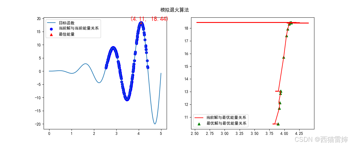
图6 极大值模拟退火算法求解
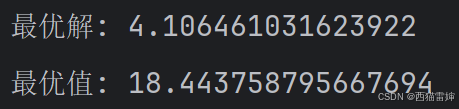
图7 极大值模拟退火算法求解控制台结果
【4】细节说明
上述内容提供了三种形式的代码,实际运行中,动画输出运行过程占用的电脑资源较多,会造成卡顿,因此选择了图片输出运行过程。
由于目标函数比较简单,因此迭代次数也较少。反复运行代码确实会出现计算不准确的情况,大家可以自由修改迭代次数等参数来提高计算准确性。
【5】总结
进一步使用python探索了模拟退火算法解决数学问题的基本技巧。


 1035
1035

 被折叠的 条评论
为什么被折叠?
被折叠的 条评论
为什么被折叠?
 到【灌水乐园】发言


