tensorflow笔记2-----实现鸢尾花分类

# -*- coding: utf-8 -*-
"""
使用tensorflow框架搭建网络实现鸢尾花分类
步骤：
1.准备数据
  ·加载数据集
  ·随机打乱数据集
  ·划分数据集：分为测试集与训练集
  ·将特征与标签匹配
2.定义网络中的每次迭代更新的参数：权值和偏置
3.使用梯度下降法更新参数，并在每一次记录测试集上的准确率
4.作出准确率的图像
"""
import tensorflow as tf
import numpy as np
from sklearn.datasets import load_iris
import matplotlib.pyplot as plt
##加载数据集
data_x=load_iris().data
data_y=load_iris().target
##随机打乱数据集
np.random.seed(100)
np.random.shuffle(data_x)
np.random.seed(100)#每一次的随机种子相同，使标签和特征匹配
np.random.shuffle(data_y)
np.random.seed(100)
##划分数据集
train_x=data_x[:-30]
train_y=data_y[:-30]
test_x=data_x[-30:]
test_y=data_y[-30:]
##转换特征的数据类型，不然运行时会因为前后数据类型不一致而出错
train_x=tf.cast(train_x,dtype=tf.float32)
test_x=tf.cast(test_x,dtype=tf.float32)
##将特征与标签匹配,每一次喂入30个训练模型
train=tf.data.Dataset.from_tensor_slices((train_x,train_y)).batch(32)
test=tf.data.Dataset.from_tensor_slices((test_x,test_y)).batch(32)
##定义网络中的参数
w=tf.Variable(tf.random.truncated_normal([4,3],stddev=0.1,seed=1))##输入特征数量为4，输出特征为3个
b=tf.Variable(tf.random.truncated_normal([3],stddev=0.1,seed=1))##偏置项，输出特征为3个
##定义存储结果的相关变量
total_epoch=500##训练次数
test_acc=[]##存储测试集上的准确率
train_loss=[]##测试集上的损失
loss_b=0##存储喂入每一batch时的损失
lr=0.1##学习率
for epoch in range(total_epoch):
    for i,(x_train,y_train) in enumerate(train):
        with tf.GradientTape() as tape:##定义计算梯度的结构
             y=tf.matmul(x_train,w)+b##输入层的输出
             y=tf.nn.softmax(y)##softmax归一化
             y_=tf.one_hot(y_train,depth=3)##将对应训练集上的标签化为one-hot形式，方便计算损失
             loss=tf.reduce_mean(tf.square(y_-y))
             loss_b+=loss.numpy()
        grad=tape.gradient(loss,[w,b])##梯度
        ##更新参数
        w.assign_sub(lr*grad[0])
        b.assign_sub(lr*grad[1])
    print("Epoch {},loss {}".format(epoch,loss_b/4))
    train_loss.append(loss_b/4)
    loss_b=0
    ##在该参数的前提下，对测试集进行预测
    correct_num,total_num=0,0
    for i,(x_test,y_test) in enumerate(test):
        y=tf.matmul(x_test,w)+b##使用更新后的参数进行预测
        y=tf.nn.softmax(y)
        pred=tf.argmax(y,axis=1)##返回分类结果对应的最大值的标签
        pred=tf.cast(pred,dtype=y_test.dtype)
        correct_num+=tf.reduce_sum(tf.cast(tf.equal(pred,y_test),dtype=tf.int32))
        total_num+=x_test.shape[0]
    ##输出准确率
    acc=correct_num/total_num
    test_acc.append(acc)
    print("Test_acc:",acc.numpy())
    print('-------------------------')
##绘制最后的图像
plt.figure(figsize=(10,8))
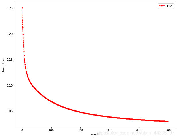
plt.xlabel('epoch')
plt.ylabel('train_loss')
plt.plot(train_loss,marker='.',color='r',linestyle='--',label="loss")
plt.legend(loc="best")
plt.show()
plt.figure(figsize=(10,8))
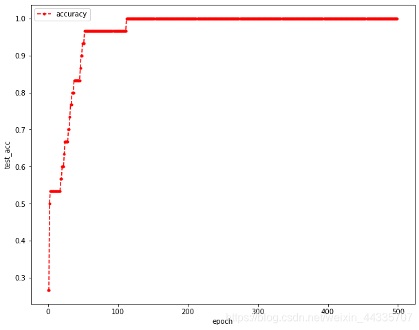
plt.xlabel('epoch')
plt.ylabel('test_acc')
plt.plot(test_acc,marker='.',color='r',linestyle='--',label="accuracy")
plt.legend(loc="best")
plt.show()  

结果如下：