《深度学习 第二章 神经网络的数学基础》

神经网络的数学基础

1.数据载入
使用python的Keras库中的手写数字数据集进行实践学习
可以从网上直接下载，下载完了，直接用load载入下载好的数据及就好了：

#from keras.datasets import mnist
#(train_images,train_labels),(test_images,test_labels) = mnist.load_data()

import numpy as np
#这里用load直接load下载好的文件
data = np.load('D:\python\workspace\mnist.npz') # open and read
print(data.keys())

这里下载下来的是.npz文件，关于.npz文件，load其实是一个字典类型的对象，整个数据延迟加载，所以变量空间里是没有显示变量的，是空的

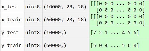
打印出这个字典类型的键值：[‘x_test’, ‘x_train’, ‘y_train’, ‘y_test’]

x_train, y_train = data['x_train'], data['y_train'] # assgian dict values
x_test, y_test = data['x_test'], data['y_test']
data.close() # close the file

这个时候变量空间有值了：

2.网络构建

#构建网络
from keras import models
from keras import layers

network = models.Sequential()
network.add(layers.Dense(512,activation = 'relu',input_shape = (28*28,)))
network.add(layers.Dense(10,activation = 'softmax'))

可能会报错：
softmax() got an unexpected keyword argument ‘axis’
去softmax()函数里面把axis参数删掉就可以了

3.编译步骤，三个参数

#编译步骤
network.compile(optimizer = 'rmsprop',loss = 'categorical_crossentropy',metrics = ['accuracy'])
#compile有三个参数：损失函数，优化器，在训练过程中需要监控的指标

4.数据预处理

#训练数据之前，对数据进行预处理
#每一个28*28的矩阵里面都是灰度值[0,255]之间，我们缩放到[0,1]之间
#训练数据是三维的60000*28*28，我们把28*28作为一个向量，变成60000*784的形状
train_images = x_train.reshape(60000,28*28)
train_images = train_images.astype('float')/255

test_images = x_test.reshape(10000,28*28)#测试数据10000条
test_images = test_images.astype('float32')/255

##准备标签
from keras.utils import to_categorical

train_labels = to_categorical(y_train)
test_labels = to_categorical(y_test)

5.训练过程

##训练过程,fit
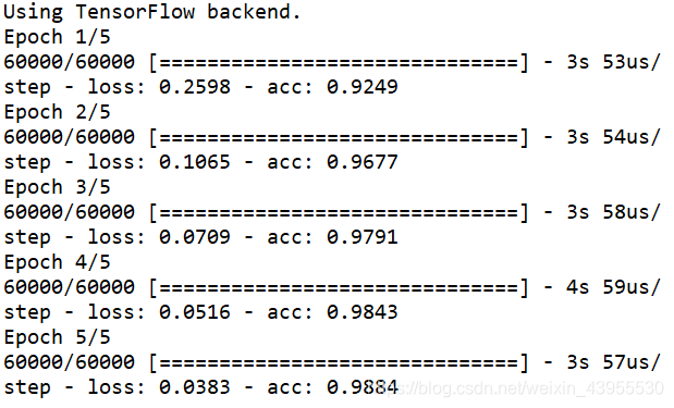
network.fit(train_images,train_labels,epochs = 5,batch_size = 128)

这里不能用y_train，一定要用train_labels，即换成独热码之后的，因为神经网络输出为10维的独热码，应该与train_labels这种十维的数进行比较
如果直接用神经网络训练出来的与y_train比较就会报错：

network.fit(train_images,y_train,epochs = 5,batch_size = 128)

ValueError: Error when checking target: expected dense_2 to have shape (10,) but got array with shape (1,)

6.结果
用cpu的tensorflow跑

用gpu的tensorflow跑：

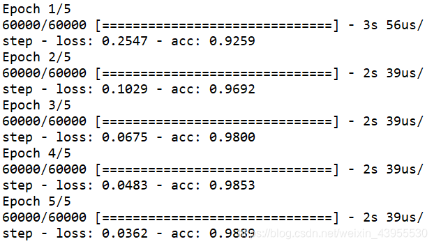
在训练集上，准确度达到了0.989
在测试机上：

test_loss,test_acc = network.evaluate(test_images,test_labels)
10000/10000 [==============================] - 0s 48us/step

print('test_acc:',test_acc)
test_acc: 0.9823

精度达到了0.9823

Code

#from keras.datasets import mnist
#(train_images,train_labels),(test_images,test_labels) = mnist.load_data()

import numpy as np
#为了避免每一次运行程序，那个下载的步骤都要进行一次，这里用load直接load下载好的文件
data = np.load('D:\python\workspace\mnist.npz') # open and read
#print(data.keys())

x_train, y_train = data['x_train'], data['y_train'] # assgian dict values
x_test, y_test = data['x_test'], data['y_test']
data.close() # close the file


#构建网络
from keras import models
from keras import layers

network = models.Sequential()
network.add(layers.Dense(512,activation = 'relu',input_shape = (28*28,)))
network.add(layers.Dense(10,activation = 'softmax'))

#编译步骤
network.compile(optimizer = 'rmsprop',loss = 'categorical_crossentropy',metrics = ['accuracy'])
#compile有三个参数：损失函数，优化器，在训练过程中需要监控的指标

#训练数据之前，对数据进行预处理
#每一个28*28的矩阵里面都是灰度值[0,255]之间，我们缩放到[0,1]之间
#训练数据是三维的60000*28*28，我们把28*28作为一个向量，变成60000*784的形状
train_images = x_train.reshape(60000,28*28)
train_images = train_images.astype('float')/255

test_images = x_test.reshape(10000,28*28)#测试数据10000条
test_images = test_images.astype('float32')/255

##准备标签
from keras.utils import to_categorical

train_labels = to_categorical(y_train)
test_labels = to_categorical(y_test)

##训练过程,fit
network.fit(train_images,train_labels,epochs = 5,batch_size = 128)
#每次处理128个样本，训练集一共60000个样本，每轮要处理469次，epochs = 5，处理五轮，一共就是进行2345次梯度更新

7.数学基础

• 张量（tensor）
  • 标量（0D张量）
  • 向量（1D张量）
  • 矩阵（2D张量）
  • 3D张量及多维张量

train_images.ndim#查看张量维数
Out[3]: 2

x_train.ndim
Out[4]: 3

x_train.shape#查看形状
Out[5]: (60000, 28, 28)

x_train.dtype#查看数据类型
Out[6]: dtype('uint8')

• Numpy中操作张量

  • 张量切片

my_slice = x_train[10:100]

• 张量广播
• 张量点积
• 张量变形

train_images = x_train.reshape(60000,28*28)

x = np.zeros((300,200))

x = np.transpose(x)

x.shape
Out[29]: (200, 300)

8.现实生活中数据张量

• 向量数据：2D张量
• 时间序列数据，序列数据：3D张量
• 图像：4D张量
• 视频：5D张量

9.神经网络的引擎
基于梯度的优化，使loss函数达到最小值，让w朝着梯度下降反方向移动

10.动量
解决陷入局部最小点而找不到全局最小点问题，和收敛速度的问题