Spark分区方式详解

最新推荐文章于 2025-05-09 14:41:55 发布

转载最新推荐文章于 2025-05-09 14:41:55 发布 · 1.6k 阅读

笔记专栏收录该内容

7 篇文章

订阅专栏

一、Spark数据分区方式简要

在Spark中，RDD（Resilient Distributed Dataset）是其最基本的抽象数据集，其中每个RDD是由若干个Partition组成。在Job运行期间，参与运算的Partition数据分布在多台机器的内存当中。这里可将RDD看成一个非常大的数组，其中Partition是数组中的每个元素，并且这些元素分布在多台机器中。图一中，RDD1包含了5个Partition，RDD2包含了3个Partition，这些Partition分布在4个节点中。

Spark包含两种数据分区方式：HashPartitioner（哈希分区）和RangePartitioner（范围分区）。一般而言，对于初始读入的数据是不具有任何的数据分区方式的。数据分区方式只作用于<Key，Value>形式的数据。因此，当一个Job包含Shuffle操作类型的算子时，如groupByKey，reduceByKey etc，此时就会使用数据分区方式来对数据进行分区，即确定某一个Key对应的键值对数据分配到哪一个Partition中。在Spark Shuffle阶段中，共分为Shuffle Write阶段和Shuffle Read阶段，其中在Shuffle Write阶段中，Shuffle Map Task对数据进行处理产生中间数据，然后再根据数据分区方式对中间数据进行分区。最终Shffle Read阶段中的Shuffle Read Task会拉取Shuffle Write阶段中产生的并已经分好区的中间数据。图2中描述了Shuffle阶段与Partition关系。下面则分别介绍Spark中存在的两种数据分区方式。

二、HashPartitioner（哈希分区）

1、HashPartitioner原理简介

HashPartitioner采用哈希的方式对<Key，Value>键值对数据进行分区。其数据分区规则为 partitionId = Key.hashCode % numPartitions，其中partitionId代表该Key对应的键值对数据应当分配到的Partition标识，Key.hashCode表示该Key的哈希值，numPartitions表示包含的Partition个数。图3简单描述了HashPartitioner的数据分区过程。

2、HashPartitioner源码详解

HashPartitioner源码较为简单，这里不再进行详细解释。


class HashPartitioner(partitions: Int) extends Partitioner {
  require(partitions >= 0, s"Number of partitions ($partitions) cannot be negative.")
 
  /**
    * 包含的分区个数
    */
  def numPartitions: Int = partitions
 
  /**
    * 获得Key对应的partitionId
    */
  def getPartition(key: Any): Int = key match {
    case null => 0
    case _ => Utils.nonNegativeMod(key.hashCode, numPartitions)
  }
 
  override def equals(other: Any): Boolean = other match {
    case h: HashPartitioner =>
      h.numPartitions == numPartitions
    case _ =>
      false
  }
 
  override def hashCode: Int = numPartitions
}
 
def nonNegativeMod(x: Int, mod: Int): Int = {
  val rawMod = x % mod
  rawMod + (if (rawMod < 0) mod else 0)
}

三、RangePartitioner（范围分区）

1、RangePartitioner原理简介

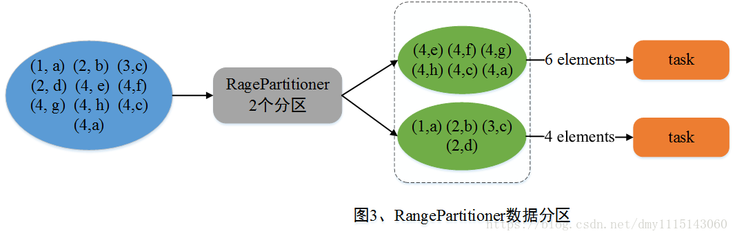
Spark引入RangePartitioner的目的是为了解决HashPartitioner所带来的分区倾斜问题，也即分区中包含的数据量不均衡问题。HashPartitioner采用哈希的方式将同一类型的Key分配到同一个Partition中，因此当某一或某几种类型数据量较多时，就会造成若干Partition中包含的数据过大问题，而在Job执行过程中，一个Partition对应一个Task，此时就会使得某几个Task运行过慢。RangePartitioner基于抽样的思想来对数据进行分区。图4简单描述了RangePartitioner的数据分区过程。

2、RangePartitioner源码详解

① 确定采样数据的规模：RangePartitioner默认对生成的子RDD中的每个Partition采集20条数据，样本数据最大为1e6条。


// 总共需要采集的样本数据个数，其中partitions代表最终子RDD中包含的Partition个数
val sampleSize = math.min(20.0 * partitions, 1e6)

② 确定父RDD中每个Partition中应当采集的数据量：这里注意的是，对父RDD中每个Partition采集的数据量会在平均值上乘以3，这里是为了后继在进行判断一个Partition是否发生了倾斜，当一个Partition包含的数据量超过了平均值的三倍，此时会认为该Partition发生了数据倾斜，会对该Partition调用sample算子进行重新采样。


// 被采样的RDD中每个partition应该被采集的数据，这里将平均采集每个partition中数据的3倍
val sampleSizePerPartition = math.ceil(3.0 * sampleSize / rdd.partitions.length).toInt

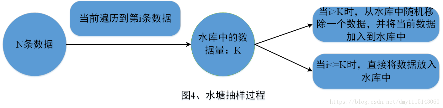
③ 调用sketch方法进行数据采样：sketch方法返回的结果为<采样RDD的数据量，<partitionId, 分区数据量，分区采样的数据量>>。在sketch方法中会使用水塘抽样算法对待采样的各个分区进行数据采样，这里采用水塘抽样算法是由于实现无法知道每个Partition中包含的数据量，而水塘抽样算法可以保证在不知道整体的数据量下仍然可以等概率地抽取出每条数据。图4简单描述了水塘抽样过程。


// 使用sketch方法进行数据抽样
val (numItems, sketched) = RangePartitioner.sketch(rdd.map(_._1), sampleSizePerPartition)
 
/**
  * @param rdd 需要采集数据的RDD
  * @param sampleSizePerPartition 每个partition采集的数据量
  * @return <采样RDD数据总量,<partitionId, 当前分区的数据量，当前分区采集的数据量>>
  */
def sketch[K : ClassTag](
    rdd: RDD[K],
    sampleSizePerPartition: Int): (Long, Array[(Int, Long, Array[K])]) = {
  val shift = rdd.id
  val sketched = rdd.mapPartitionsWithIndex { (idx, iter) =>
    val seed = byteswap32(idx ^ (shift << 16))
    // 使用水塘抽样算法进行抽样，抽样结果是个二元组<Partition中抽取的样本量，Partition中包含的数据量>
    val (sample, n) = SamplingUtils.reservoirSampleAndCount(
      iter, sampleSizePerPartition, seed)
    Iterator((idx, n, sample))
  }.collect()
  val numItems = sketched.map(_._2).sum
  (numItems, sketched)
}

④ 数据抽样完成后，需要对不均衡的Partition重新进行抽样，默认当Partition中包含的数据量大于平均值的三倍时，该Partition是不均衡的。当采样完成后，利用样本容量和RDD中包含的数据总量，可以得到整体的一个数据采样率fraction。利用此采样率对不均衡的Partition调用sample算子重新进行抽样。


// 计算数据采样率
val fraction = math.min(sampleSize / math.max(numItems, 1L), 1.0)
// 存放采样Key以及采样权重
val candidates = ArrayBuffer.empty[(K, Float)]
// 存放不均衡的Partition
val imbalancedPartitions = mutable.Set.empty[Int]
//（idx, n, sample）=> (partition id, 当前分区数据个数，当前partition的采样数据)
sketched.foreach { case (idx, n, sample) =>
  // 当一个分区中的数据量大于平均分区数据量的3倍时，认为该分区是倾斜的
  if (fraction * n > sampleSizePerPartition) {
    imbalancedPartitions += idx
  }
  // 在三倍之内的认为没有发生数据倾斜
  else {
    // 每条数据的采样间隔 = 1/采样率 = 1/(sample.size/n.toDouble) = n.toDouble/sample.size
    val weight = (n.toDouble / sample.length).toFloat
    // 对当前分区中的采样数据，对每个key形成一个二元组<key, weight>
    for (key <- sample) {
      candidates += ((key, weight))
    }
  }
}
// 对于非均衡的partition，重新采用sample算子进行抽样
if (imbalancedPartitions.nonEmpty) {
  val imbalanced = new PartitionPruningRDD(rdd.map(_._1), imbalancedPartitions.contains)
  val seed = byteswap32(-rdd.id - 1)
  val reSampled = imbalanced.sample(withReplacement = false, fraction, seed).collect()
  val weight = (1.0 / fraction).toFloat
  candidates ++= reSampled.map(x => (x, weight))
}

⑤ 确定各个Partition的Key范围：使用determineBounds方法来确定每个Partition中包含的Key范围，先对采样的Key进行排序，然后计算每个Partition平均包含的Key权重，然后采用平均分配原则来确定各个Partition包含的Key范围。如当前采样Key以及权重为：<1, 0.2>, <2, 0.1>, <3, 0.1>, <4, 0.3>, <5, 0.1>, <6, 0.3>，现在将其分配到3个Partition中，则每个Partition的平均权重为：（0.2 + 0.1 + 0.1 + 0.3 + 0.1 + 0.3） / 3 = 0.36。此时Partition1 ~ 3分配的Key以及总权重为<Partition1, {1, 2, 3}, 0.4> <Partition2, {4, 5}, 0.4> <Partition1, {6}, 0.3>。


/**
  * @param candidates 未按采样间隔排序的抽样数据
  * @param partitions 最终生成的RDD包含的分区个数
  * @return 分区边界
  */
def determineBounds[K : Ordering : ClassTag](
    candidates: ArrayBuffer[(K, Float)],
    partitions: Int): Array[K] = {
  val ordering = implicitly[Ordering[K]]
  // 对样本按照key进行排序
  val ordered = candidates.sortBy(_._1)
  // 抽取的样本容量
  val numCandidates = ordered.size
  // 抽取的样本对应的采样间隔之和
  val sumWeights = ordered.map(_._2.toDouble).sum
  // 平均每个分区的步长
  val step = sumWeights / partitions
  var cumWeight = 0.0
  var target = step
  // 分区边界值
  val bounds = ArrayBuffer.empty[K]
  var i = 0
  var j = 0
  var previousBound = Option.empty[K]
  while ((i < numCandidates) && (j < partitions - 1)) {
    val (key, weight) = ordered(i)
    cumWeight += weight
    // 当前的采样间隔小于target，继续迭代，也即这些key应该放在同一个partition中
    if (cumWeight >= target) {
      // Skip duplicate values.
      if (previousBound.isEmpty || ordering.gt(key, previousBound.get)) {
        bounds += key
        target += step
        j += 1
        previousBound = Some(key)
       }
    }
    i += 1
  }
  bounds.toArray
}

⑥ 计算每个Key所在Partition：当分区范围长度在128以内，使用顺序搜索来确定Key所在的Partition，否则使用二分查找算法来确定Key所在的Partition。


/**
  * 获得每个Key所在的partitionId
  */
def getPartition(key: Any): Int = {
  val k = key.asInstanceOf[K]
  var partition = 0
  // 如果得到的范围不大于128，则进行顺序搜索
  if (rangeBounds.length <= 128) {
    // If we have less than 128 partitions naive search
    while (partition < rangeBounds.length && ordering.gt(k, rangeBounds(partition))) {
      partition += 1
    }
  }
  // 范围大于128，则进行二分搜索该key所在范围，即可得到该key所在的partitionId
  else {
    // Determine which binary search method to use only once.
    partition = binarySearch(rangeBounds, k)
    // binarySearch either returns the match location or -[insertion point]-1
    if (partition < 0) {
      partition = -partition-1
    }
    if (partition > rangeBounds.length) {
      partition = rangeBounds.length
    }
  }
  if (ascending) {
    partition
  } else {
    rangeBounds.length - partition
  }
}

                    <h1><a name="t0"></a>一、Spark数据分区方式简要 &nbsp;&nbsp;&nbsp;&nbsp;&nbsp;</h1>