0-4.正则化（Regularization），合理初始化权重，梯度校验

最新推荐文章于 2025-04-06 20:23:26 发布

我不是坏人...真的

最新推荐文章于 2025-04-06 20:23:26 发布

阅读量759

点赞数

分类专栏：饿

本文链接：https://blog.youkuaiyun.com/weixin_43668325/article/details/102523355

版权

饿专栏收录该内容

14 篇文章

订阅专栏

本文深入探讨了深度学习中常见的问题及解决方案，包括梯度消失与爆炸的缓解方法，正则化技术如L2和dropout的应用，以及梯度校验的重要性。通过合理初始化权值、正则化和梯度校验，可以显著提升模型的稳定性和泛化能力。

摘要生成于 C知道，由 DeepSeek-R1 满血版支持，前往体验 >

训练集和测试集：GitHub上的Desktop.rar中GitHub链接

本文中讲的内容有：（完整代码在文章底部）

（1）.合理初始化权值，缓解随着神经网络层数增加产生的梯度爆炸与消失问题。

（2）.正则化（缓解过拟合现象）：L2正则化（权重衰减）—对应文件Ragularization_L2.py。dropout正则化（反向随机失活）—对应文件Regularization_dropout.py。还有L1正则化，early stopping正则化，数据扩增等。

（3）.梯度校验。

一.合理初始化权值：

1.梯度消失与梯度爆炸产生的原因：

对于深层神经网络，计算图是先经过线性函数z = w.a+b，然后在经过激活函数，重复多次构成的。
我们假设b=0，激活函数是一个线性函数f（z）=z。
此时y^ = w1.w2.w3…wL*X (注意w是矩阵)。
为了方便计算，假设w矩阵中除主对角线外的元素都是0，且主对角线元素都相等，即将w矩阵看成比单位矩阵略大一点点或者略小一点点。
在这里插入图片描述

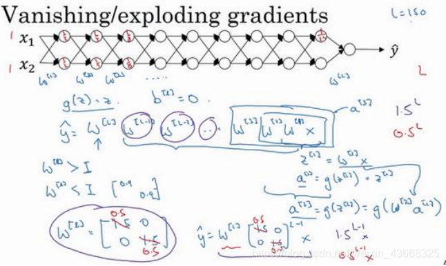
当w是比单位矩阵略小一点点时，不妨设为0.9：此时：y ^ = 0.9^LX,激活函数呈指数形式递减。当w是比单位矩阵略大一点点时，不妨设为1.1；此时：y ^=1.1 ^L X,激活函数呈指数形式爆炸式递增。

我们只讨论了激活函数情况，对于关于其他关于L层的函数和导数也有这个特性。如果对于一个很深的深层神经网络来说，激活函数呈爆炸式增加或减小，将会使梯度下降算法的步长变得很小，导致梯度下降算法学习十分缓慢。这也是前文中如果将神经网络层数L设为6层7层比较深的时候前文链接，需要训练很多轮模型才会有效。下面我们来缓解这个现象。

	如果你想用 Relu 激活函数，也就是最常用的激活函数，我会用这个公式np. sqrt( 2 /?[?−1])；
	如果使用 tanh 函数，可以用公式np.sqrt(1 /?[?−1])。
	w = np.random.randn(dim, m) * np.sqrt(2 / m)
	w = np.random.randn(dim, m) * np.sqrt(1 / m)

我们将初始化w和b的代码改成这样：

def ward(L,n,m,dim):#对参数进行初始化
    np.random.seed(1)
    w = []
    b = []
    for i in range(0, L):
        if i != 0 and i != L - 1:
            # p = np.random.randn(dim, dim) *0.001
            p = np.random.randn(dim, dim) * np.sqrt(2 / dim)
        elif i == 0:
            # p = np.random.randn(dim, m) * 0.001
            p = np.random.randn(dim, m) * np.sqrt(2 / m)
        else:
            # p = np.random.randn(1, dim) * 0.001
            p = np.random.randn(1, dim) * np.sqrt(2 / dim)
        w.append(p)
        b.append(1)

    return w,b

二.正则化：

1.L2正则化：减小权重w的值，使得取值落在激活函数相对线性的部分，让神经网络变得更简单，这是L2正则化有效的原因。L2正则化改变损失函数J的定义，在前向传播过程中往损失函数增加权值w矩阵的范数之和与正则化参数的乘积，超参数为lambd（通常取0.01量级）。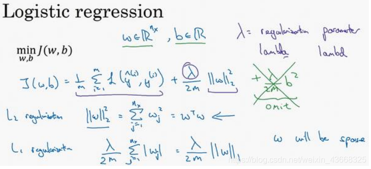

前反向传播需要更改的代码：

def forward(w,b,a,Y,L,m,lambd):#前向传播
    z = []
    J = 0
    add = 0
    for i in range(0, L):
        zl = np.dot(w[i], a) + b[i]
        add += np.sum((lambd / (2 * m)) * np.dot(w[i], w[i].T))#L2正则化项
        z.append(zl)
        a = relu(zl)
    a = sigmoid(zl)

    J = (-1/m)*np.sum(1 * Y * np.log(a) + (1 - Y) * np.log(1 - a)) + add  # 损失函数
    return z, a, J
def backward(w,b,X,Y,learning,m,L,lambd):#反向传播
    z,a,J = forward(w,b,X,Y,L,m,lambd)

    for i in range(L - 1, 0, -1):
        if i == L - 1:
            dz = a - Y
        else:
            dz = np.dot(w[i + 1].T, dz) * relu_1(z[i])
        dw = 1 / m * (np.dot(dz, relu(z[i - 1]).T)) + (lambd / m) * w[i]
        db = 1 / m * np.sum(dz, axis=1, keepdims=True)
        w[i] -= learning * dw
        b[i] -= learning * db

        # b[i] = np.mean(b[i] - learning*db)
    dz = np.dot(w[1].T, dz) * relu_1(z[0])
    dw = 1 / m * np.dot(dz, X.T) + (lambd / m) * w[0]
    db = 1 / m * np.sum(dz, axis=1, keepdims=True)

    w[0] -= learning * dw
    b[0] -= learning * db
    # b[0] = np.mean(b[0] - learning*db)
    return w, b, J

运行结果：

在这里插入图片描述

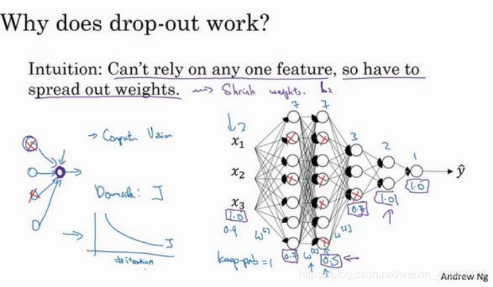
2.dropout正则化：通过消去神经元使得神经网络变得简单，这是dropout有效的原因。dropout正则化随机消去指定的某一层的神经元，超参数为keep_prob（通常取0.8，但必须为0.5到1之间的数，通常比较接近1；取1时相当于关闭dropout正则化）,消除层的位置可以任取，每一层的keep_prob取值也可以不同。

注意：(1).因为随机消去神经元，所以损失函数J将没有明确定义，无法分析损失函数，调试时候通常关闭dropout正则化；(2).测试时候不用经过dropout正则化。

在这里插入图片描述
dropout正则化代码实现：

d3 = np.random.rand(a3.shape[0],a3.shape[1]) < keep_prob
a3 = np.multiply(a3,d3)
a3 = a3 / keep_prob

dropout正则化前反向传播需要更改的代码：

def forward1(w,b,a,Y,L,m,dL,keep_prob):#前向传播
    z = []
    J = 0
    for i in range(0,L):
        zL = np.dot(w[i],a) + b[i]
        z.append(zL)
        a = relu(zL)
        if i < 2 or i==L-1:#增加dorpout正则化项
            p = np.random.rand(a.shape[0],a.shape[1]) < 1
            dL.append(p)
            a = np.multiply(a,p)/1
        else:
            p = np.random.rand(a.shape[0], a.shape[1]) < keep_prob
            dL.append(p)
            a = np.multiply(a, p)/keep_prob
    a = sigmoid(zL)
    J = (-1/m)*np.sum(1 * Y * np.log(a) + (1 - Y) * np.log(1 - a))#损失函数
    return z,a,J,dL
def backward(w,b,X,Y,learning,m,L,keep_prob):#反向传播
    dL = []#表示消除的神经元，是一个布尔值矩阵
    z,a,J,dL = forward1(w,b,X,Y,L,m,dL,keep_prob)

    for i in range(L-1,0,-1):
        if i == L-1:
            dz = a-Y
        else:
            dz = np.dot(w[i+1].T,dz)*(relu_1(z[i])*dL[i])
        dw = 1/m * np.dot(dz,(relu(z[i-1])*dL[i]).T)
        db = 1/m * np.sum(dz,axis=1,keepdims=True)
        w[i] -= learning*dw
        b[i] -= learning*db

        #b[i] = np.mean(b[i] - learning*db)
    dz = np.dot(w[1].T,dz)*(relu_1(z[0])*dL[0])
    dw = 1/m * np.dot(dz,X.T)
    db = 1/m * np.sum(dz,axis=1,keepdims=True)

    w[0] -= learning*dw
    b[0] -= learning * db
    #b[0] = np.mean(b[0] - learning*db)
    return w,b,J

运行结果：

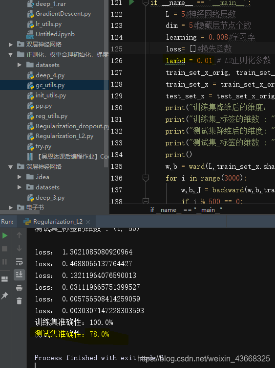
(1).keep_prob取0.9时：测试集结果为80%

在这里插入图片描述

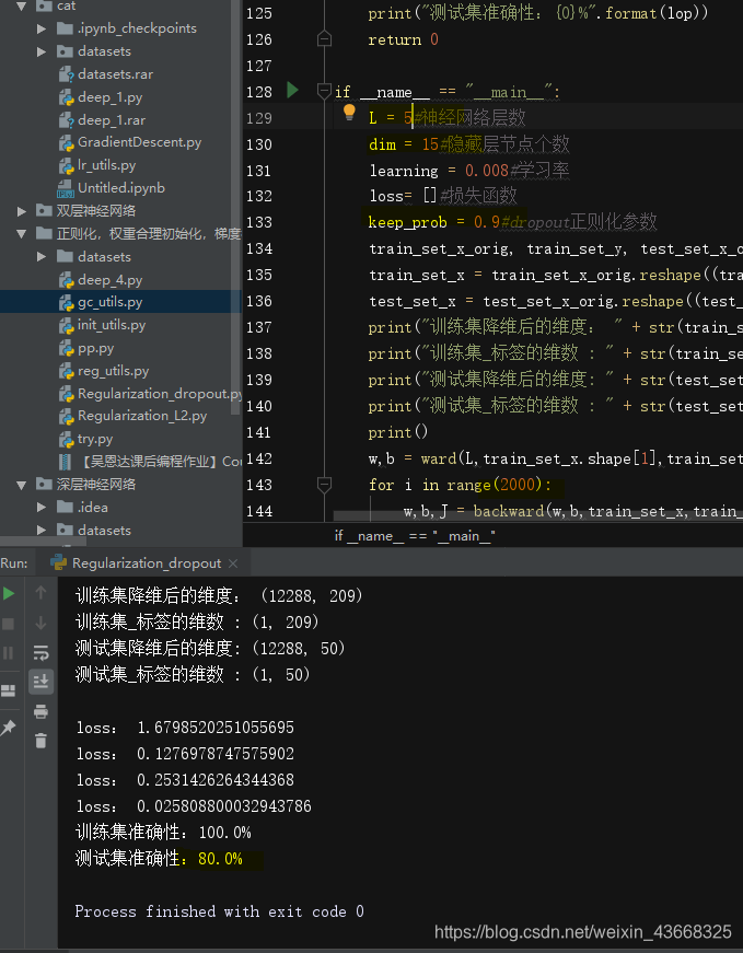
(2).keep_prob取0.8时：，测试集结果为82%

在这里插入图片描述

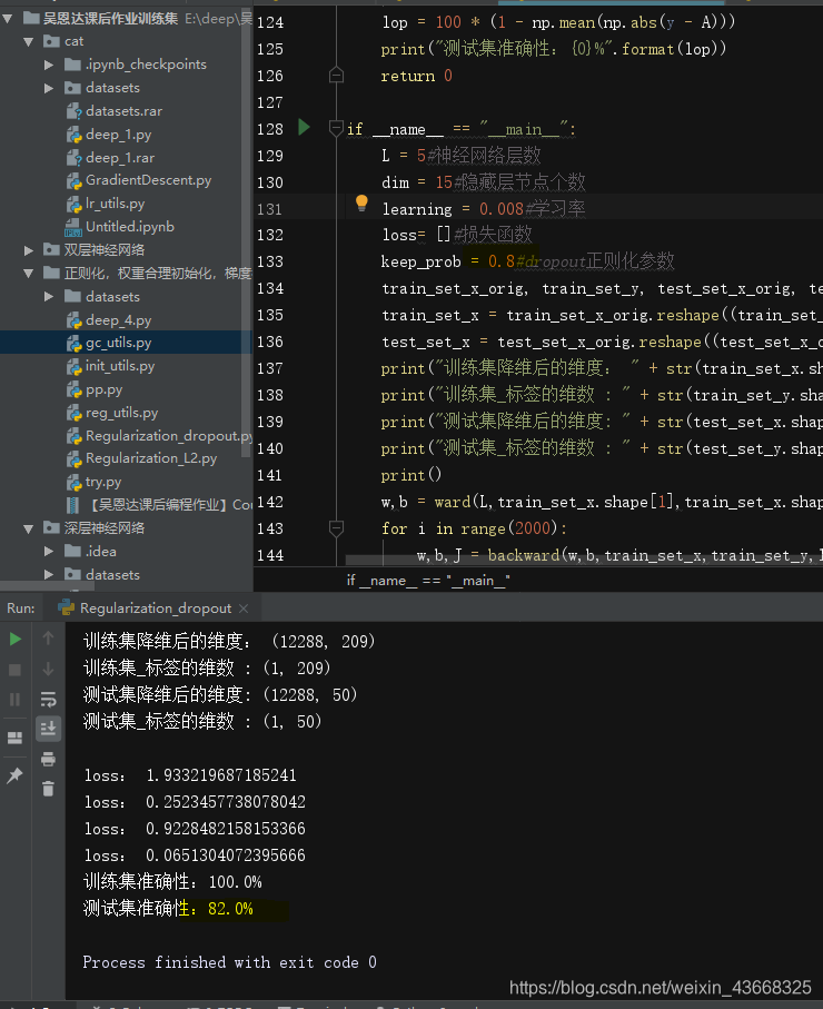
更改参数的值，结果也会不同，可能准确率更高也可能更低，大家可以多调试；显而易见的是，dropout正则化和L2正则化使得神经网络变得更简单了,缓解了过拟合现象问题；较之前文中的三层神经网络需要训练5000轮，训练轮数明显减少了也能达到同样效果。

三.梯度校验：

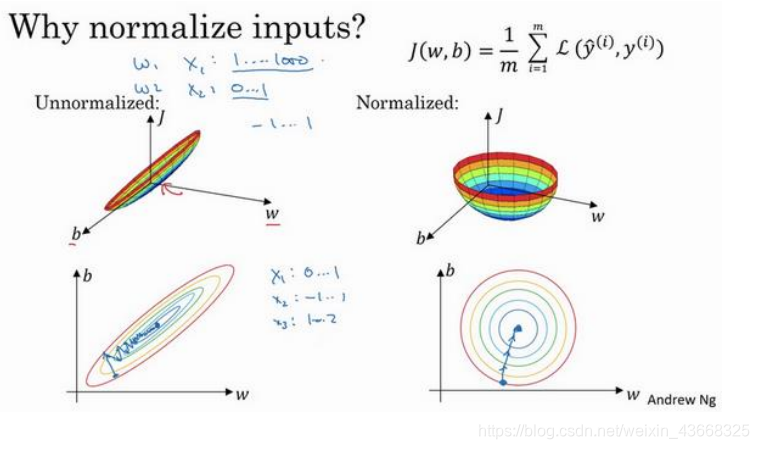
1.归一化输入：

训练神经网络，其中一个加速训练的方法就是归一化输入。假设一个训练集有两个特征，
输入特征为 2 维，归一化需要两个步骤：
（1）.零均值
（2）.归一化方差

在这里插入图片描述

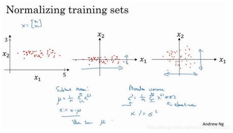
(1).第一步是零均值化，? 它是一个向量，?等于每个训练数据 ?减去?，意思是移动训练集，直到它完成零均值化。
(2).第二步是归一化方差，注意特征?1的方差比特征?2的方差要大得多，我们要做的是给?
赋值，这是节点? 的平方，?2是一个向量，它的每个特征都有方差，注意，我们已经完成零值均化，(?(?))2元素?2就是方差，我们把所有数据除以向量?2，最后变成上图形式(其实就是求方差?2)。

2.实施梯度校验（调试使用）：

在这里插入图片描述
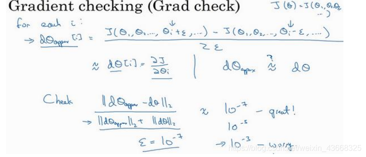
假设你的网络中含有下列参数，?[1]和?[1]……?[?]和?[?]，为了执行梯度检验，首先要做
的就是，把所有参数转换成一个巨大的向量数据，你要做的就是把矩阵?转换成一个向量，
把所有?矩阵转换成向量之后，做连接运算，得到一个巨型向量?，该向量表示为参数?，代
价函数?是所有?和?的函数，现在你得到了一个?的代价函数?（即?(?)）。接着，你得到与
?和?顺序相同的数据，你同样可以把??[1]和??[1]……??[?]和??[?]转换成一个新的向量，用
它们来初始化大向量??，它与?具有相同维度。
同样的，把??[1]转换成矩阵，??[1]已经是一个向量了，直到把??[?]转换成矩阵，这样
所有的??都已经是矩阵，注意??[1]与?[1]具有相同维度，??[1]与?[1]具有相同维度。经过
相同的转换和连接运算操作之后，你可以把所有导数转换成一个大向量??，它与?具有相同
维度。为了实施梯度检验，你要做的就是循环执行，从而对每个?也就是对每个?组成元素计
算??approx[?]的值，我使用双边误差，也就是
??approx[?] = （?(?1, ?2,… ?? + ?, … )−?(?1, ?2,… ?? − ?, … )）/2?
只对??增加?，其它项保持不变，因为我们使用的是双边误差，对另一边做同样的操作，
只不过是减去?，?其它项全都保持不变。
计算这两个向量的距离，??approx[?] − ??[?]的欧几里得范数，注意这里（||??approx − ??||）没有平方，它是误差平方之和，然后求平方根，得到欧式距离，然后用向量长度归一化，使用向量长度的
欧几里得范数。分母只是用于预防这些向量太小或太大，分母使得这个方程式变成比率，我
们实际执行这个方程式，?可能为10^−7，使用这个取值范围内的?，如果你发现计算方程式得
到的值为10^−7或更小，这就很好，这就意味着导数逼近很有可能是正确的，它的值非常小。
如果它的值在10^−5范围内，我就要小心了，也许这个值没问题，但我会再次检查这个向
量的所有项，确保没有一项误差过大，可能这里有 bug。
如果左边这个方程式结果是10^−3，我就会担心是否存在 bug，计算结果应该比10^−3小很
多，如果比10^−3大很多，我就会很担心，担心是否存在 bug。这时应该仔细检查所有?项，
看是否有一个具体的?值，使得??approx[?]与??[?]大不相同，并用它来追踪一些求导计算是否正确，经过一些调试，最终结果会是这种非常小的值（10^−7），那么，你的实施可能是正
确的。

3.梯度检验应用的注意事项：

	第一点，不要在训练中使用梯度检验，它只用于调试。
	第二点，如果算法的梯度检验失败，要检查所有项，检查每一项，并试着找出 bug，也
就是说，如果??approx[?]与??[?]的值相差很大，我们要做的就是查找不同的?值，看看是哪个
导致??approx[?]与??[?]的值相差这么多。
	第三点，在实施梯度检验时，如果使用正则化，请注意正则项。??等于与?相关的?函数的梯度，
包括这个正则项，记住一定要包括这个正则项。
	第四点，梯度检验不能与 dropout 同时使用，因为每次迭代过程中，dropout 会随机消
除隐藏层单元的不同子集，难以计算 dropout 在梯度下降上的代价函数?。
	第五点，也是比较微妙的一点，现实中几乎不会出现这种情况。当?和?接近 0 时，
梯度下降的实施是正确的，在随机初始化过程中……，但是在运行梯度下降时，?和?变得更
大。可能只有在?和?接近 0 时，backprop 的实施才是正确的。但是当?和?变大时，它会变
得越来越不准确。你需要做一件事，我不经常这么做，就是在随机初始化过程中，运行梯度
检验，然后再训练网络，?和?会有一段时间远离 0，如果随机初始化值比较小，反复训练网
络之后，再重新运行梯度检验。

Regularization_L2.py:

# conding:utf-8
import numpy as np
import matplotlib.pyplot as plt
import h5py
def load_dataset():
    train_dataset = h5py.File('datasets/train_catvnoncat.h5', "r")
    train_set_x_orig = np.array(train_dataset["train_set_x"][:])  # 保存的是训练集里面的图像数据（本训练集有209张64x64的图像）。
    train_set_y_orig = np.array(train_dataset["train_set_y"][:])  # 保存的是训练集的图像对应的分类值（【0 | 1】，0表示不是猫，1表示是猫）。
    test_dataset = h5py.File('datasets/test_catvnoncat.h5', "r")
    test_set_x_orig = np.array(test_dataset["test_set_x"][:])  # 保存的是测试集里面的图像数据（本训练集有50张64x64的图像）。
    test_set_y_orig = np.array(test_dataset["test_set_y"][:])  # 保存的是测试集的图像对应的分类值（【0 | 1】，0表示不是猫，1表示是猫）。
    classes = np.array(test_dataset["list_classes"][:])  # 保存的是以bytes类型保存的两个字符串数据，数据为：[b’non-cat’ b’cat’]。
    train_set_y = train_set_y_orig.reshape((1, train_set_y_orig.shape[0]))
    test_set_y = test_set_y_orig.reshape((1, test_set_y_orig.shape[0]))

    print("训练集_图片的维数 : " + str(train_set_x_orig.shape))
    print("训练集_标签的维数 : " + str(train_set_y.shape))
    print("测试集_图片的维数: " + str(test_set_x_orig.shape))
    print("测试集_标签的维数: " + str(test_set_y.shape))
    print()
    return train_set_x_orig, train_set_y, test_set_x_orig, test_set_y, classes
def tanh(z):#tanh函数
    return (np.exp(z)-np.exp(-z))/(np.exp(z)+np.exp(-z))
def relu(z):#relu函数
    return np.maximum(0,z)
def tanh_1(z):#tanh函数的导数
    return 1-tanh(z)**2
def relu_1(z):#relu函数的导数
    return np.maximum(0, z/np.abs(z))
def sigmoid(z):
    return 1/(1+np.exp(-z))

def ward(L,n,m,dim):#对参数进行初始化
    np.random.seed(1)
    w = []
    b = []
    for i in range(0, L):
        if i != 0 and i != L - 1:
            #p = np.random.randn(dim, dim) *0.001
            p = np.random.randn(dim, dim) * np.sqrt(2 / dim)
        elif i == 0:
            #p = np.random.randn(dim, m) * 0.001
            p = np.random.randn(dim, m) * np.sqrt(2 / m)
        else:
            #p = np.random.randn(1, dim) * 0.001
            p = np.random.randn(1, dim) * np.sqrt(2 / dim)
        w.append(p)
        b.append(1)
    '''
    w1 = np.random.randn(t,m)
    w2 = np.random.randn(L-2,t,t)#隐藏层重复部分参数，第一维存层数减2，第二维下一层节点个数t，第三维存当前层节点个数t
    w3 = np.random.randn(1,t)
    w = {
        "w1":w1,
        "w2":w2,
        "w3":w3
    }
    b = np.zeros(shape = (L,1,1),dtype = 'float')
    '''
    return w, b

def forward(w,b,a,Y,L,m,lambd):#前向传播
    z = []
    J = 0
    add = 0
    for i in range(0, L):
        zl = np.dot(w[i], a) + b[i]
        add += np.sum((lambd / (2 * m)) * np.dot(w[i], w[i].T))#L2正则化项
        z.append(zl)
        a = relu(zl)
    a = sigmoid(zl)

    J = (-1/m)*np.sum(1 * Y * np.log(a) + (1 - Y) * np.log(1 - a)) + add  # 损失函数
    return z, a, J
def backward(w,b,X,Y,learning,m,L,lambd):#反向传播
    z,a,J = forward(w,b,X,Y,L,m,lambd)

    for i in range(L - 1, 0, -1):
        if i == L - 1:
            dz = a - Y
        else:
            dz = np.dot(w[i + 1].T, dz) * relu_1(z[i])
        dw = 1 / m * (np.dot(dz, relu(z[i - 1]).T)) + (lambd / m) * w[i]
        db = 1 / m * np.sum(dz, axis=1, keepdims=True)
        w[i] -= learning * dw
        b[i] -= learning * db

        # b[i] = np.mean(b[i] - learning*db)
    dz = np.dot(w[1].T, dz) * relu_1(z[0])
    dw = 1 / m * np.dot(dz, X.T) + (lambd / m) * w[0]
    db = 1 / m * np.sum(dz, axis=1, keepdims=True)

    w[0] -= learning * dw
    b[0] -= learning * db
    # b[0] = np.mean(b[0] - learning*db)
    return w, b, J


def train(x,y,w,b,L,m,lambd):#查看训练集准确率
    A = np.zeros(shape=(1, x.shape[1]))
    z, a,J = forward(w, b, x, y,L,m,lambd)

    for i in range(x.shape[1]):
        # A.append(0 if a[0,i] <0.5 else 1)
        A[0, i] = 0 if a[0, i] < 0.5 else 1
    lop = 100 * (1 - np.mean(np.abs(y - A)))
    print("训练集准确性：{0}%".format(lop))
    return 0

def text(x,y,w,b,L,m,lambd):#查看测试集准确率
    A = np.zeros(shape=(1, x.shape[1]))
    z, a,J = forward(w, b, x, y, L, m,lambd)

    for i in range(x.shape[1]):
        # A.append(0 if a[0,i] <0.5 else 1)
        A[0, i] = 0 if a[0, i] < 0.5 else 1
    lop = 100 * (1 - np.mean(np.abs(y - A)))
    print("测试集准确性：{0}%".format(lop))
    return 0

if __name__ == "__main__":
    L = 5#神经网络层数
    dim = 5#隐藏层节点个数
    learning = 0.008#学习率
    loss= []#损失函数
    lambd = 0.01 # L2正则化参数
    train_set_x_orig, train_set_y, test_set_x_orig, test_set_y, classes = load_dataset()
    train_set_x = train_set_x_orig.reshape((train_set_x_orig.shape[0], -1)).T / 255  # 降维,化为区间（0，1）内的数
    test_set_x = test_set_x_orig.reshape((test_set_x_orig.shape[0], -1)).T / 255  # 降维,化为区间（0，1）内的数
    print("训练集降维后的维度： " + str(train_set_x.shape))
    print("训练集_标签的维数 : " + str(train_set_y.shape))
    print("测试集降维后的维度: " + str(test_set_x.shape))
    print("测试集_标签的维数 : " + str(test_set_y.shape))
    print()
    w,b = ward(L,train_set_x.shape[1],train_set_x.shape[0],dim)
    for i in range(3000):
        w,b,J = backward(w,b,train_set_x,train_set_y,learning,train_set_x.shape[1],L,lambd)
        if i % 500 == 0:
            print("loss：",J)
            loss.append(J)
    plt.plot(loss)#打印损失函数
    plt.show()
    train(train_set_x,train_set_y,w,b,L,train_set_x.shape[1],lambd)
    text(test_set_x,test_set_y,w,b,L,test_set_x.shape[1],lambd)

Regularization_dropout.py:

# conding:utf-8
import numpy as np
import matplotlib.pyplot as plt
import h5py
def load_dataset():
    train_dataset = h5py.File('datasets/train_catvnoncat.h5', "r")
    train_set_x_orig = np.array(train_dataset["train_set_x"][:])  # 保存的是训练集里面的图像数据（本训练集有209张64x64的图像）。
    train_set_y_orig = np.array(train_dataset["train_set_y"][:])  # 保存的是训练集的图像对应的分类值（【0 | 1】，0表示不是猫，1表示是猫）。
    test_dataset = h5py.File('datasets/test_catvnoncat.h5', "r")
    test_set_x_orig = np.array(test_dataset["test_set_x"][:])  # 保存的是测试集里面的图像数据（本训练集有50张64x64的图像）。
    test_set_y_orig = np.array(test_dataset["test_set_y"][:])  # 保存的是测试集的图像对应的分类值（【0 | 1】，0表示不是猫，1表示是猫）。
    classes = np.array(test_dataset["list_classes"][:])  # 保存的是以bytes类型保存的两个字符串数据，数据为：[b’non-cat’ b’cat’]。
    train_set_y = train_set_y_orig.reshape((1, train_set_y_orig.shape[0]))
    test_set_y = test_set_y_orig.reshape((1, test_set_y_orig.shape[0]))

    print("训练集_图片的维数 : " + str(train_set_x_orig.shape))
    print("训练集_标签的维数 : " + str(train_set_y.shape))
    print("测试集_图片的维数: " + str(test_set_x_orig.shape))
    print("测试集_标签的维数: " + str(test_set_y.shape))
    print()
    return train_set_x_orig, train_set_y, test_set_x_orig, test_set_y, classes
def tanh(z):#tanh函数
    return (np.exp(z)-np.exp(-z))/(np.exp(z)+np.exp(-z))
def relu(z):#relu函数
    return np.maximum(0,z)
def tanh_1(z):#tanh函数的导数
    return 1-tanh(z)**2
def relu_1(z):#relu函数的导数
    return np.maximum(0, z/np.abs(z))
def sigmoid(z):
    return 1/(1+np.exp(-z))

def ward(L,n,m,dim):#对参数进行初始化
    np.random.seed(1)
    w = []
    b = []
    for i in range(0, L):
        if i != 0 and i != L - 1:
            # p = np.random.randn(dim, dim) *0.001
            p = np.random.randn(dim, dim) * np.sqrt(2 / dim)
        elif i == 0:
            # p = np.random.randn(dim, m) * 0.001
            p = np.random.randn(dim, m) * np.sqrt(2 / m)
        else:
            # p = np.random.randn(1, dim) * 0.001
            p = np.random.randn(1, dim) * np.sqrt(2 / dim)
        w.append(p)
        b.append(1)

    return w,b

def forward1(w,b,a,Y,L,m,dL,keep_prob):#前向传播
    z = []
    J = 0
    for i in range(0,L):
        zL = np.dot(w[i],a) + b[i]
        z.append(zL)
        a = relu(zL)
        if i < 2 or i==L-1:#增加dorpout正则化项
            p = np.random.rand(a.shape[0],a.shape[1]) < 1
            dL.append(p)
            a = np.multiply(a,p)/1
        else:
            p = np.random.rand(a.shape[0], a.shape[1]) < keep_prob
            dL.append(p)
            a = np.multiply(a, p)/keep_prob
    a = sigmoid(zL)

    J = (-1/m)*np.sum(1 * Y * np.log(a) + (1 - Y) * np.log(1 - a))#损失函数
    return z,a,J,dL
def forward2(w,b,a,Y,L,m):#测试时使用的前向传播
    z = []
    J = 0
    for i in range(0,L):
        zl = np.dot(w[i],a) + b[i]
        z.append(zl)
        a = relu(zl)
    a = sigmoid(zl)

    J = (-1/m)*np.sum(1 * Y * np.log(a) + (1 - Y) * np.log(1 - a))#损失函数
    return z,a,J
def backward(w,b,X,Y,learning,m,L,keep_prob):#反向传播
    dL = []#表示消除的神经元，是一个布尔值矩阵
    z,a,J,dL = forward1(w,b,X,Y,L,m,dL,keep_prob)

    for i in range(L-1,0,-1):
        if i == L-1:
            dz = a-Y
        else:
            dz = np.dot(w[i+1].T,dz)*(relu_1(z[i])*dL[i])
        dw = 1/m * np.dot(dz,(relu(z[i-1])*dL[i]).T)
        db = 1/m * np.sum(dz,axis=1,keepdims=True)
        w[i] -= learning*dw
        b[i] -= learning*db

        #b[i] = np.mean(b[i] - learning*db)
    dz = np.dot(w[1].T,dz)*(relu_1(z[0])*dL[0])
    dw = 1/m * np.dot(dz,X.T)
    db = 1/m * np.sum(dz,axis=1,keepdims=True)

    w[0] -= learning*dw
    b[0] -= learning * db
    #b[0] = np.mean(b[0] - learning*db)
    return w,b,J

def train(x,y,w,b,L,m):#查看训练集准确率
    A = np.zeros(shape=(1, x.shape[1]))
    z, a,J = forward2(w, b, x, y,L,m)

    for i in range(x.shape[1]):
        # A.append(0 if a[0,i] <0.5 else 1)
        A[0, i] = 0 if a[0, i] < 0.5 else 1
    lop = 100 * (1 - np.mean(np.abs(y - A)))
    print("训练集准确性：{0}%".format(lop))
    return 0

def text(x,y,w,b,L,m):#查看测试集准确率
    A = np.zeros(shape=(1, x.shape[1]))
    z, a,J = forward2(w, b, x, y, L, m)

    for i in range(x.shape[1]):
        # A.append(0 if a[0,i] <0.5 else 1)
        A[0, i] = 0 if a[0, i] < 0.5 else 1
    lop = 100 * (1 - np.mean(np.abs(y - A)))
    print("测试集准确性：{0}%".format(lop))
    return 0

if __name__ == "__main__":
    L = 5#神经网络层数
    dim = 15#隐藏层节点个数
    learning = 0.008#学习率
    loss= []#损失函数
    keep_prob = 0.8#dropout正则化参数
    train_set_x_orig, train_set_y, test_set_x_orig, test_set_y, classes = load_dataset()
    train_set_x = train_set_x_orig.reshape((train_set_x_orig.shape[0], -1)).T / 255  # 降维,化为区间（0，1）内的数
    test_set_x = test_set_x_orig.reshape((test_set_x_orig.shape[0], -1)).T / 255  # 降维,化为区间（0，1）内的数
    print("训练集降维后的维度： " + str(train_set_x.shape))
    print("训练集_标签的维数 : " + str(train_set_y.shape))
    print("测试集降维后的维度: " + str(test_set_x.shape))
    print("测试集_标签的维数 : " + str(test_set_y.shape))
    print()
    w,b = ward(L,train_set_x.shape[1],train_set_x.shape[0],dim)
    for i in range(2000):
        w,b,J = backward(w,b,train_set_x,train_set_y,learning,train_set_x.shape[1],L,keep_prob)
        if i % 500 == 0:
            print("loss：",J)
            loss.append(J)
    plt.plot(loss)
    plt.show()
    train(train_set_x,train_set_y,w,b,L,train_set_x.shape[1])
    text(test_set_x,test_set_y,w,b,L,test_set_x.shape[1])