


1. Introduction
大部分的刚体机器人可以看成是连杆耦合的,倒立摆是最基本的结构,研究倒立摆有助于理解后面的章节。
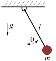
刚体的运动方程,一般通过拉格朗日方法获取更为方便。
m
l
2
θ
¨
(
t
)
+
m
g
l
s
i
n
θ
(
t
)
=
Q
ml^2\ddot{\theta}(t)+mglsin\theta(t)=Q
ml2θ¨(t)+mglsinθ(t)=Q
Q可以看成是广义力,控制输入u+摩擦力产生的转矩。
Q
=
−
b
θ
˙
(
t
)
+
u
(
t
)
Q = -b\dot{\theta}(t)+u(t)
Q=−bθ˙(t)+u(t)
2.2 Nonlinear dynamics with a constant torque
这显然是一个非线性的问题,哪怕最简单的形式:
q
˙
=
a
q
→
q
(
t
)
=
q
(
0
)
e
a
t
\dot{q}=aq \to q(t)=q(0)e^{at}
q˙=aq→q(t)=q(0)eat
对于这样的系统,根据a来判断:
1)a<0, exponential decay, 最终稳定;
2)a=0,系统不动;
3)a>0,exponential growing, 不稳定状态。
控制系统中有很多的技术可以根据a来判断是否稳定,如根轨迹法、bode图等。
2.2.1 the overdamped pendulum(一阶系统)
引入工具前,先简化系统。对于典型的二阶倒立摆
m
l
2
θ
¨
+
b
θ
˙
+
m
g
l
θ
=
0
ml^2\ddot{\theta}+b\dot{\theta}+mgl\theta=0
ml2θ¨+bθ˙+mglθ=0
固有频率为
w
n
=
g
l
w_n=\sqrt{\frac{g}{l}}
wn=lg,阻尼系数
ζ
=
b
2
m
l
2
l
g
\zeta=\frac{b}{2ml^2}\sqrt{\frac{l}{g}}
ζ=2ml2bgl。
当
b
θ
˙
>
>
m
l
2
θ
¨
,
b
∗
l
g
>
>
m
l
2
b\dot{\theta}>>ml^2\ddot{\theta},b*\sqrt{\frac{l}{g}}>>ml^2
bθ˙>>ml2θ¨,b∗gl>>ml2,这是个大阻尼的系统,就像在蜜罐中运动。
b
θ
˙
=
u
0
−
m
g
l
s
i
n
(
θ
)
b\dot{\theta}=u_0-mglsin(\theta)
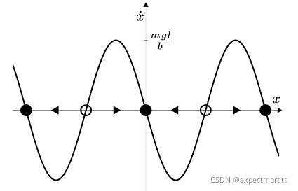
bθ˙=u0−mglsin(θ)
- matlab 绘制
通过采样 θ = − 10 : 0.01 : 10 \theta=-10:0.01:10 θ=−10:0.01:10,很方便绘制出这样的轨迹。

当
x
˙
=
0
,
\dot{x}=0,
x˙=0,被成为fixed point;但是fixed point也会有两种
1)unstable,只要稍微离开了平衡点,就被自身的动力学拉的越来越远;
2)locally stable, 只要到了locally stable的区间,最终会达到平衡状态。
对于locally stable,有三种定义
1)李雅普诺夫稳定,通俗的理解,对于一个半径为
ϵ
\epsilon
ϵ的球,只要初始的状态在半径为
δ
\delta
δ的球中,系统会一直保持在
ϵ
\epsilon
ϵ的球内。
i
.
s
.
l
s
t
a
b
l
e
:
→
∀
ϵ
>
0
,
∃
δ
,
满
足
∣
∣
x
(
0
)
−
x
∗
∣
∣
<
δ
,
使
得
∀
∣
∣
x
(
t
)
−
x
∗
∣
∣
<
ϵ
i.s.l \quad stable: \to \quad \forall \, \epsilon >0,\exist \delta, \\ 满足||x(0)-x^{*}||<\delta, 使得\forall ||x(t)-x^{*}||<\epsilon
i.s.lstable:→∀ϵ>0,∃δ,满足∣∣x(0)−x∗∣∣<δ,使得∀∣∣x(t)−x∗∣∣<ϵ
2)locally attractive, 也是上图上表现的,即使一开始和目标点有误差,最终也会渐进到x*。
i
f
x
(
0
)
=
x
∗
+
ϵ
→
l
i
m
t
→
∞
x
(
t
)
=
x
∗
if\, x(0)=x^*+\epsilon \quad \to \quad lim_{t \to \infty}x(t)=x^*
ifx(0)=x∗+ϵ→limt→∞x(t)=x∗
3)locally asymptotically stable,如果一个fixed point 同时满足上述两个条件。
4)locally exponentially stable,状态是指数收敛到目标值。
i
f
x
(
0
)
=
x
∗
+
ϵ
,
→
∣
∣
x
(
t
)
−
x
∗
∣
∣
<
C
e
−
a
t
if \, x(0)=x^*+\epsilon, \quad \to \quad ||x(t)-x^*||<Ce^{-at}
ifx(0)=x∗+ϵ,→∣∣x(t)−x∗∣∣<Ce−at
李雅普诺夫只要误差满足在一个范围内就行,attractive需要渐进到目标点。asymptocally stable最终会达到目标点,exponentially stable以一定的速率达到目标点。
注意事项:
1)attractive并不意味着i.s.l stable:
r
˙
=
r
(
1
−
r
)
θ
˙
=
s
i
n
2
(
θ
/
2
)
\begin{aligned} \dot{r} &=r(1-r) \\ \dot{\theta} & = sin^2(\theta/2) \end{aligned}
r˙θ˙=r(1−r)=sin2(θ/2)
在r*=1, θ = 0 \theta=0 θ=0也是attract point,但是并不是stable的。
继续分析单个倒立摆的状态图,可以看到
1)在x=0点附近是asymptocally stable,甚至是exponentially stable(最起码收敛的速度是快于线性切线拟合系统的速率);
2)对于x=0.
[
−
π
,
π
]
[-\pi, \pi]
[−π,π]被称为basin of attraction,就是说只要初始在这个basin中,最终系统都会到目标点x=0;
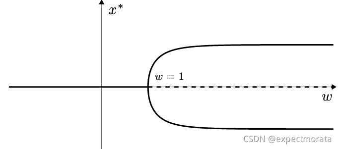
- bifurcation
系统的稳定点很多时候是受系统参数的影响,换言之收到控制量 u 0 u_0 u0的影响。
例如,对于系统 x ˙ + x = t a n h ( w x ) \dot{x}+x=tanh(wx) x˙+x=tanh(wx)
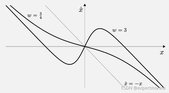
w和稳定点数目之间的关系如下图,w=1就是bifurcation(分歧点)。
2.2.2 The undamped pendulum(二阶系统)
但是实际机器人系统往往都是二阶系统,上面那些表示不能完整表达系统的动力学关系。
方法是phase portrait,看代码很容易理解。
m
l
2
θ
¨
=
u
0
−
m
g
l
s
i
n
(
θ
)
−
b
θ
ml^2\ddot{\theta}=u_0-mglsin(\theta)-b\theta
ml2θ¨=u0−mglsin(θ)−bθ
拆解成
[
θ
˙
θ
¨
]
=
[
0
1
0
−
b
m
l
2
]
[
θ
θ
˙
]
+
[
0
−
g
s
i
n
(
θ
)
l
]
\begin{aligned} \begin{bmatrix} \dot{\theta} \\ \ddot{\theta} \end{bmatrix} = \begin{bmatrix} 0 & 1 \\ 0 & -\frac{b}{ml^2} \end{bmatrix} \begin{bmatrix} \theta \\ \dot{\theta} \end{bmatrix} + \begin{bmatrix} 0\\ -\frac{gsin(\theta)}{l} \end{bmatrix} \end{aligned}
[θ˙θ¨]=[001−ml2b][θθ˙]+[0−lgsin(θ)]
step1:将
(
θ
,
θ
˙
)
(\theta, \dot{\theta})
(θ,θ˙)写成meshgrid的形式,然后计算
(
θ
˙
,
θ
¨
)
(\dot{\theta},\ddot{\theta})
(θ˙,θ¨),就是对应的向量。
step2:找几个初始点,用ode45跑个一段时间,绘制轨迹;从图上也能看出来ode45绘制出来的轨迹和向量方向相同的。
% phase portait
clear all; close all; clc
f = @(t,Y) [Y(2); -sin(Y(1))];
y1 = linspace(-2,8,20);
y2 = linspace(-2,2,20);
[x,y] = meshgrid(y1,y2);
u = zeros(size(x));
v = zeros(size(x));
t=0; % we want the derivatives at each point at t=0, i.e. the starting time
for i = 1:numel(x)
    Yprime = f(t,[x(i); y(i)]);
    u(i) = Yprime(1);
    v(i) = Yprime(2);
end

quiver(x,y,u,v,'r'); figure(gcf)
xlabel('y_1')
ylabel('y_2')
axis tight equal;
hold on
for y20 = [0 0.5 1 1.5 2 2.5]
    [ts,ys] = ode45(f,[0,50],[0;y20]);
    plot(ys(:,1),ys(:,2))
    plot(ys(1,1),ys(1,2),'bo') % starting point
    plot(ys(end,1),ys(end,2),'ks') % ending point
end
hold off
axis([-10 10 -5 5])
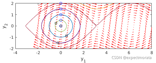
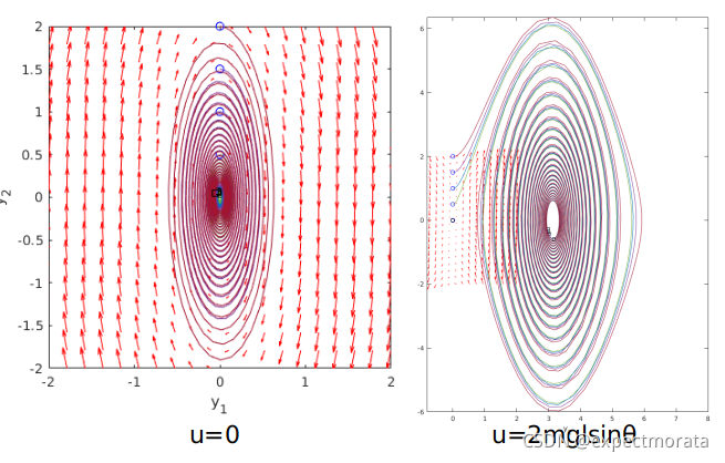
分别绘制u=0,和
u
=
2
m
g
l
s
i
n
(
θ
)
u=2mglsin(\theta)
u=2mglsin(θ)情况下的曲线,这两个的输入从物理上来看一个是重力方向向下,一个是重力方向向上如图。
2.3 The torque limited simple pendulum
如果力矩不受限制,可以将fix point 改到任意点。现实当中,关节的力矩往往收到约束的,倒立摆要想达到最高点,需要通过能量积蓄,最终达到最高点。
2.3.1 Energy-shaping control
为了将倒立摆弄到最高点,搞一个能量层面的pd控制器。
E
d
=
m
g
l
E
=
0.5
m
l
2
θ
˙
2
−
m
g
l
c
o
s
(
θ
)
E
˙
=
m
l
2
θ
˙
θ
¨
+
m
g
l
s
i
n
(
θ
)
θ
˙
=
θ
˙
(
u
−
m
g
l
s
i
n
θ
)
+
m
g
l
s
i
n
θ
θ
˙
=
θ
˙
u
\begin{aligned} E^d &=mgl \\ E & = 0.5ml^2\dot{\theta}^2-mglcos(\theta) \\ \dot{E} &=ml^2\dot{\theta}\ddot{\theta}+mglsin(\theta)\dot{\theta}\\ & = \dot{\theta}(u-mglsin\theta)+mglsin\theta \dot{\theta} \\ & = \dot{\theta}u \end{aligned}
EdEE˙=mgl=0.5ml2θ˙2−mglcos(θ)=ml2θ˙θ¨+mglsin(θ)θ˙=θ˙(u−mglsinθ)+mglsinθθ˙=θ˙u
用最基本的PD控制器,
u
=
−
k
p
(
E
−
E
d
)
=
−
k
p
θ
˙
E
~
u =-k_p(E-E^d)=-k_p \dot{\theta} \tilde{E}
u=−kp(E−Ed)=−kpθ˙E~,有
E
~
˙
=
−
k
p
θ
˙
2
E
~
\dot{\tilde{E}}=-k_p\dot{\theta}^2\tilde{E}
E~˙=−kpθ˙2E~
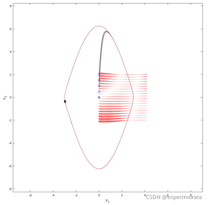
这个控制器在
E
d
E^d
Ed是attractive的,看一下phase portrait, 显然不是i.s.l stable(李雅普诺夫稳定),但是轨道却是稳定了,从这个点进行延伸就是period stable的概念了。


 被折叠的 条评论
为什么被折叠?
被折叠的 条评论
为什么被折叠?
 到【灌水乐园】发言


