从零开始手撕线性回归：代码实战带你深入理解机器学习基础

从零开始手撕线性回归：代码实战带你深入理解机器学习基础

线性回归是机器学习中最基础且重要的算法之一，广泛应用于预测分析和数据建模。本文将带领读者从零开始理解线性回归的核心原理，并通过Python代码实战一步步实现一个简单的线性回归模型。无论你是机器学习初学者还是希望巩固基础的开发者，本文都将为你提供清晰的学习路径。

线性回归是一种监督学习算法，用于建立输入变量（特征）与输出变量（目标）之间的线性关系。其核心思想是找到一条最佳拟合直线，使得预测值与真实值之间的误差最小。假设我们有一组数据点 (x, y)，线性回归试图找到参数 w 和 b，使得以下公式成立：
$$y=wx+b$$
其中，w 是权重（表示特征对目标的影响程度），b 是偏置（表示目标值的基准）。为了衡量模型的拟合效果，我们通常使用均方误差（MSE）作为损失函数：
$$MSE=\frac{1}{n}\sum _{i=1}^n(y_i-{\hat{y}}_i{)}^2$$

实验代码

import random
import torch
from typing import Union, Tuple
import matplotlib.pyplot as plt


def synthetic_data(w: torch.Tensor, b: float, num_examples: int) -> Tuple[torch.Tensor, torch.Tensor]:
    """
    根据w和b生成线性回归曲线y
    :param w: 权重参数
    :param b: 偏执项
    :param num_examples: 样本的数量
    :return:
    """
    X = torch.normal(0, 1, (num_examples, len(w)))
    y = torch.matmul(X, w) + b
    y += torch.normal(0, 0.01, y.shape)
    return X, y.reshape((-1, 1))


def data_iter(batch_size: int, features: torch.Tensor, labels: torch.Tensor) -> Tuple[torch.Tensor, torch.Tensor]:
    """
    生成器获取数据集
    :param batch_size: 小批量大小
    :param features: 特征矩阵X
    :param labels: 标签Y
    :return:
    X, Y

    """
    num_examples = len(features)
    indices = list(range(num_examples))
    # 这些样本是随机读取的，没有特定的顺序
    random.shuffle(indices)
    for i in range(0, num_examples, batch_size):
        batch_indices = torch.tensor(
            indices[i: min(i + batch_size, num_examples)])
        yield features[batch_indices], labels[batch_indices]


def linreg(X, w, b):
    """
    线性回归模型
    y = w*x+b
    """
    return torch.matmul(X, w) + b


def sgd(params, lr, batch_size):
    """
    随机梯度下降优化器
    :param:params 权重参数w
    :param:lr 学习lv
    :param:batch_size 批量大小
    """
    with torch.no_grad():
        for param in params:
            param -= lr * param.grad / batch_size
            param.grad.zero_()


def squared_loss(y_hat: torch.Tensor, y: torch.Tensor) -> torch.Tensor:
    """
    均方损失函数
    :param: y_hat 预测值
    :param: y 真实值
    :return
    损失值
    """
    return (y_hat - y.reshape(y_hat.shape)) ** 2 / 2


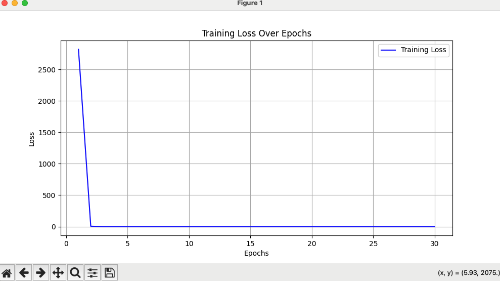
def plt_loss(loss_list: list):
    """
    画损失值随epoch变化图
    :param loss_list:
    :return:
    """
    plt.figure(figsize=(10, 5))
    epochs = list(range(1, len(loss_list) + 1))
    # 绘制损失随轮次变化的折线图
    plt.plot(epochs, loss_list, label='Training Loss', color='blue')

    # 添加标题和坐标轴标签
    plt.title('Training Loss Over Epochs')
    plt.xlabel('Epochs')
    plt.ylabel('Loss')

    # 显示网格
    plt.grid(True)

    # 添加图例
    plt.legend()

    # 展示图形
    plt.show()


def main():
    true_w = torch.tensor([2, -3.4])
    true_b = 4.2
    # 获取样本X和真实的标签值
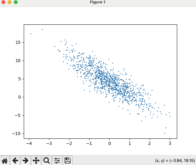
    features, labels = synthetic_data(true_w, true_b, 1000)

    # 画真实值的散点图
    plt.scatter(features[:, (1,)].detach().numpy(), labels.detach().numpy(), 1)
    plt.show()
    plt.close()

    batch_size = 10
    # 初始化w和b
    w = torch.normal(0, 0.01, size=(2, 1), requires_grad=True)
    b = torch.zeros(1, requires_grad=True)
    lr = 0.03
    num_epochs = 30
    net = linreg
    loss = squared_loss
    loss_list = []
    for epoch in range(num_epochs):
        i = 0
        total_loss = 0
        for X, y in data_iter(batch_size, features, labels):
            i += 1
            l = loss(net(X, w, b), y).sum()
            total_loss += l.item()
            print(f"train epoch:{epoch + 1} batch:{i} loss:{l}")
            # 反向传播自动计算梯度
            l.backward()
            # 使用优化器将梯度更新到参数w和b中
            sgd([w, b], lr, batch_size)
        loss_list.append(total_loss)
        with torch.no_grad():
            train_l = loss(net(features, w, b), labels)
            print(f'val epoch {epoch + 1}, loss {float(train_l.mean()):f}')
    plt_loss(loss_list)


if __name__ == '__main__':
    main()