【数据分析】Kaggle项目之共享单车数据分析（二）

数据分析

逐项展示

时段对租赁数量的影响

workingday_df=Bike_data[Bike_data['workingday']==1]
workingday_df=workingday_df.groupby(['hour'],as_index=True).agg({
    'casual':'mean','registered':'mean','count':'mean'})
nworkingday_df=Bike_data[Bike_data['workingday']==0]
nworkingday_df=nworkingday_df.groupby(['hour'],as_index=True).agg({
    'casual':'mean','registered':'mean','count':'mean'})

fig,axes=plt.subplots(1,2,sharey=True)
workingday_df.plot(figsize=(15,5),title='The average number of rentals initiated per hour in the working day',ax=axes[0])
nworkingday_df.plot(figsize=(15,5),title='The average number of rentals initiated per hour in the nonworkingdays',ax=axes[1])

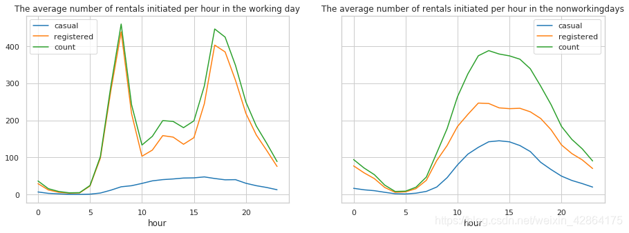
可以看出：

• 工作日对于会员用户的上下班时间是两个用车高峰，而中午也会有一个小高峰，猜测可能是外出午餐的人。
• 对于临时用户起伏比较缓慢，高峰期在17点左右
• 会员用户的用车数量远超过临时用户
• 对于非工作日而言的租赁数量随着时间呈现一个正态分布，高峰在14点左右，低谷在4点左右，且分布比较均匀

温度对租赁数量的影响

# 数据按照小时统计展示起来太麻烦，希望能够按天汇总取一天的气温中位数
temp_df = Bike_data.groupby(['date','weekday'],as_index=False).agg({'year':'mean','month':'mean','temp':'median'})
# 由于测试数据集中没有租赁信息，会导致折线图有断裂，所以将缺失的数据丢弃
temp_df.dropna(axis=0,how='any',inplace=True)
# 预计按天统计的波动仍然很大，再按月按日取平均值
temp_month=temp_df.groupby(['year','month'],as_index=False).agg({'weekday':'min','temp':'median'})
# 将按天求和统计数据的日期转换成datetime格式
temp_df['date']=pd.to_datetime(temp_df['date'])
# 将按月统计数据设置一列时间序列
temp_month.rename(columns={'weekday':'day'},inplace=True)
temp_month['date']=pd.to_datetime(temp_month[['year','month','day']])
# 设置画框尺寸
fig=plt.figure(figsize=(18,6))
ax=fig.add_subplot(1,1,1)
# 使用折线图展现总体租赁情况（count）随时间的走势
plt.plot(temp_df['date'],temp_df['temp'],linewidth=1.3,label='Daily average')
ax.set_title('Change trend of average temperature per day in two years')
plt.plot(temp_month['date'],temp_month['temp'],marker='o',linewidth=1.3,label='Monthly average')
ax.legend()

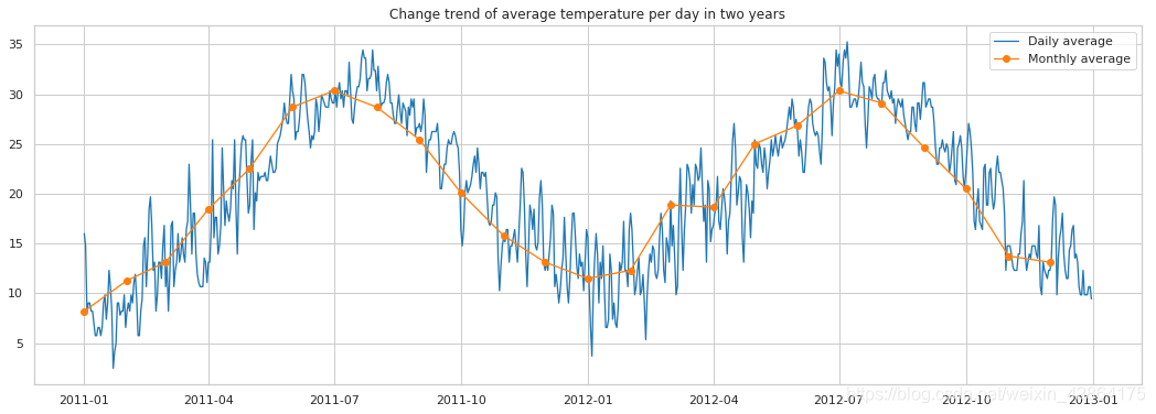
可以看出

• 每年的气温趋势相同，随着月份发生变化
• 7月份气温最高，1月份气温最低