吴恩达-机器学习课后题06-SVM(支持向量机)2-线性不可分2-寻找最优gamma

1、问题

找出最优化gamma

2、解题

1、导入数据

mat = sio.loadmat(path)
# print(mat.keys())
X,y = mat['X'],mat['y']
Xval,yval = mat['Xval'],mat['yval']#验证集

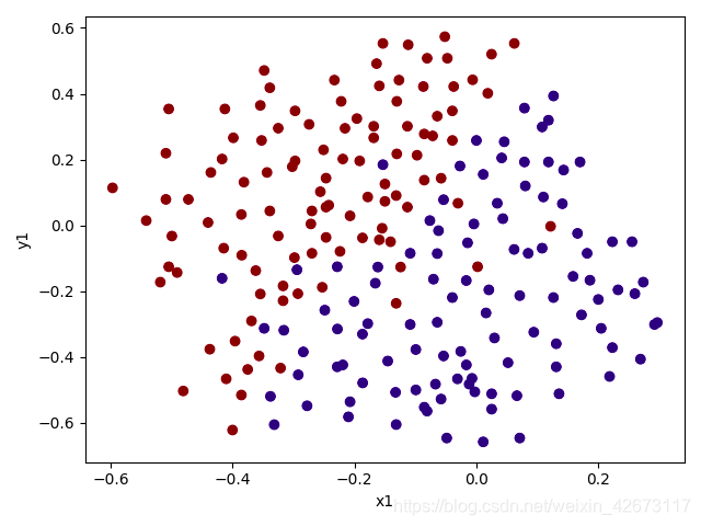
2、数据可视化：

#数据可视化
def plot_data():
    plt.scatter(X[:,0],X[:,1],c=y.flatten(),cmap='jet')
    plt.xlabel('x1')
    plt.ylabel('y1')
    plt.show()
plot_data()

结果：

3、寻找最优gamma与C

#取值:
def findBest():
    Cvalues = [0.01, 0.03, 0.1, 0.3, 1, 3, 10, 30, 100]
    gammas = [0.01, 0.03, 0.1, 0.3, 1, 3, 10, 30, 100]
    best_score = 0
    best_param = (0, 0)
    for c in Cvalues:
        for gamma in gammas:
            svc = SVC(C=c,kernel='rbf',gamma=gamma)
            svc.fit(X,y.flatten())
            score = svc.score(Xval,yval.flatten())
            if(score>=best_score):
                best_score = score
                best_param = (c,gamma)
                print(best_param,best_score)
    return best_score,best_param
best_score,best_param = findBest()

结果：
(0.1, 30) 0.95
(0.3, 10) 0.955
(0.3, 30) 0.96
(0.3, 100) 0.965
(1, 100) 0.965
(3, 30) 0.965
(30, 10) 0.965
没啥技术含量就不解释了
但是我们发现，最优的C与gamma有几种组合结果都是相同的

4、显示边界

svc2 = SVC(C=0.3,kernel='rbf',gamma=100)
svc2.fit(X,y.flatten())
def plot_boundary(model):
    x_min,x_max = -1,1
    y_min,y_max = -0.8,0.4
    xx,yy = np.meshgrid(np.linspace(x_min,x_max,500),
                        np.linspace(y_min,y_max,500))
    z = model.predict(np.c_[xx.flatten(),yy.flatten()])
    zz = z.reshape(xx.shape)
    plt.contour(xx,yy,zz)
plot_boundary(svc2)
plot_data()

结果：

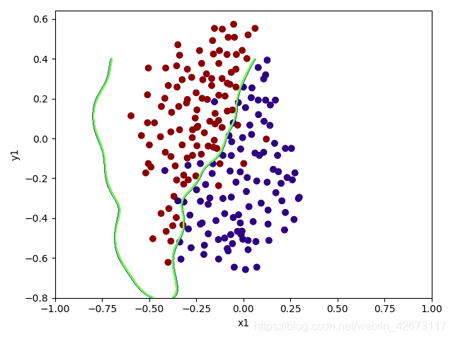
可以看出基本都区分开了