吴恩达-机器学习课后题03-神经网络实现手写数字识别-使用BP神经网络优化权重theta

1、题目

同上一篇

2、预先知识学习

1、One-hot编码

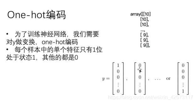
对数组进行处理，将每一位数组用一个数组10个数字表示，若第一个数字是1，表示当前数组为1，第十个数组为1，表示数字10

使用原因：因为损失函数要沿用之前的损失函数公式，之前公式中y只有0和1两种状态，所以要对其进行处理

2、对于反向传播的理解：

## 3、解题
1、导入数据

data = sio.loadmat(path)
X = data['X']
y = data['y']
X = np.insert(X,0,values=1,axis=1)

2、one-hot编码

#one-hot编码
def one_hot_encoder(y):
    result = []
    for i in y:
        y_temp = np.zeros(10)
        y_temp[i-1]=1
        result.append(y_temp)
    return np.array(result)

print(one_hot_encoder(y))
print(y)

3、序列化权重参数
因为后期会用到scipy的子模块进行最优化所以需要传入序列化的theta
需要传入的参数形式是(n,)
目前的状态：(25，401)

theta = sio.loadmat(thetaPath)
# print(theta.keys())
theta1 = theta['Theta1']
theta2 = theta['Theta2']

def serialize(a,b):
    return np.append(a.flatten(),b.flatten())

theta_sericalize = serialize(theta1,theta2)
# print(theta_sericalize.size)

序列化实质上是将两个数组进行展平，成为一位数组之后一个拼接在另外一个后面

4、解序列化
将序列化之后的数组传入，然后按之前的每一维度的大小，将其进行拆分然后reshape成原来的维度

def deSerialize(theta_serialize):
    theta1 = theta_serialize[:25*401].reshape(25,401)
    theta2 = theta_serialize[25*401:].reshape(10,26)
    return theta1,theta2

5、前向传播
调用之前的前向传播，用于计算出最后的结果h

#前向传播
def sigmoid(z):
    return 1/(1+np.exp(-z))

def feed_forword(theta_serialize,X):
    theta1,theta2 =deSerialize(theta_serialize)
    # print(theta1.shape,theta2.shape)
    a1 = X
    z2 = a1@theta1.T
    a2 = sigmoid(z2)
    a2 = np.insert(a2,0,values=1,axis=1)
    z3 = a2@theta2.T
    h = sigmoid(z3)
    return a1,z2,a2,z3,h

6、代价函数计算(正则化和不带正则化两种方法)

#定义损失函数
#1、不带正则化
def cost(theta_serialize,X,y):
    a1,z2,a2,z3,h = feed_forword(theta_serialize,X)
    J = -np.sum(y*np.log(h)+(1-y)*np.log(1-h))/len(X)
    return J
print(cost(theta_serialize,X,y))
#2、带正则化
def reg_cost(theta_serialize,X,y,lamda):
    # a1, z2, a2, z3, h = feed_forword(theta_serialize, X)
    # J = -np.sum(y * np.log(h) + (1 - y) * np.log(1-h)) / len(X)
    sum1 = np.sum(np.power(theta1[:,1:],2))
    sum2 = np.sum(np.power(theta2[:,1:],2))
    reg = (sum1+sum2)*lamda/(2*len(X))
    return cost(theta_serialize,X,y)+reg

可以看出，代价函数同样是计算最终结果和理想值的偏差

7、使用反向传播得出梯度
理解反向传播：

#定义梯度,反向传播
#1、无正则化
def sigmoid_gradient(z):
    return sigmoid(z)*(1-sigmoid(z))
def gradient(theta_serialize,X,y):
    theta1,theta2 = deSerialize(theta_serialize)
    a1,z2,a2,z3,h = feed_forword(theta_serialize,X)
    d3 = h-y
    d2 = d3@theta2[:,1:]*sigmoid_gradient(z2)
    D2 = (d3.T@a2)/len(X)
    D1 = (d2.T@a1)/len(X)
    return serialize(D1,D2)
def reg_gradient(theta_serialize,X,y,lamda):
    D = gradient(theta_serialize,X,y)
    D1,D2 = deSerialize(D)
    theta1,theta2 = deSerialize(theta_serialize)
    D1[:,1:] = D1[:,1:]+theta1[:,1:]*lamda/len(X)
    D2[:,1:] = D2[:,1:] + theta2[:, 1:] * lamda / len(X)
    return serialize(D1,D2)

反向传播就是从最后一项开始，不断使用y-求出的结果记为delta，然后对其求反导，逐步向前
用误差值不断调整参数theta

8、使用scipy中的minimize通过梯度对代价函数最小化

def nn_training(X,y):
     init_theta = np.random.uniform(-0.5,0.5,10285)
     res = so.minimize(fun=reg_cost,
                       x0=init_theta,
                       args=(X,y,lamda),
                       method='TNC',
                       jac=reg_gradient,
                       options={'maxiter':300})
     return res

注意，Python中参数外面的变量为全局变量，所以lamda可以不用传入方法即可在方法之内使用

9、对调整之后的参数带入，然后计算其准确率

lamda = 10
res = nn_training(X,y)
y = data['y'].reshape(5000,)
_,_,_,_,h = feed_forword(res.x,X)
y_pred = np.argmax(h,axis=1)+1
acc = np.mean(y_pred==y)
print(acc)

10、可视化隐藏层

def plot_hidden_layer(theta_serialize):
    theta1,_ = deSerialize(theta_serialize)
    hiden_layer = theta1[:,1:] #theta1本身是一个（25，400）的矩阵

    #使用之前使用过的显示100张图片的方法进行显示
    fig, ax = plt.subplots(ncols=5, nrows=5, figsize=(8, 8), sharex=True, sharey=True)
    plt.xticks([])
    plt.yticks([])
    for r in range(5):
        for c in range(5):
            ax[r, c].imshow(hiden_layer[5 * r + c].reshape(20, 20).T, cmap='gray_r')
    plt.show()
plot_hidden_layer(theta_serialize)

结果：

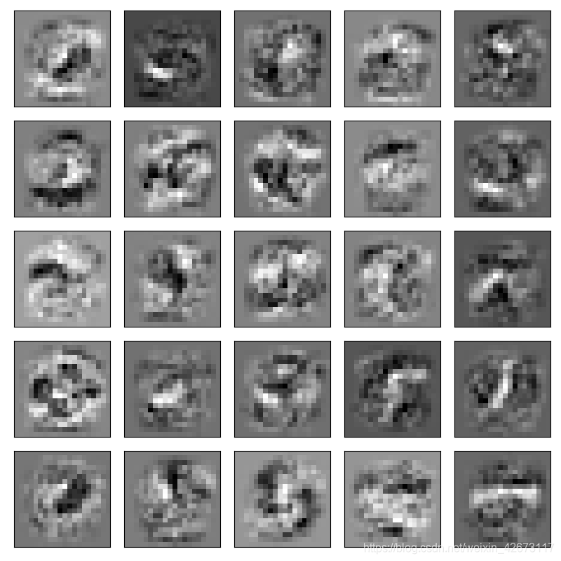
模模糊糊，其实也看不出啥来，😺