python统计套利_基于python的统计套利实战（二）之协整检验

协整关系协整(Cointegration)理论是恩格尔(Engle)和格兰杰(Granger)在1978年提出的。平稳性是进行时间序列分析的一个很重要的前提，很多模型都是基于平稳下进行的，而现实中，很多时间序列都是非平稳的，所以协整是从分析时间序列的非平稳性入手的。

协整的内容是：

设序列X是 d 阶单整的，记为X∼I(d)，如果存在一个非零向量β使得Y=βXt∼I(d−b)，则称Xt具有 d, b 阶协整关系，记为Xt∼CI(d,b)，则 β称为协整向量。

特别当 X 和 Y 都是一阶单整时，一般而言,X和 Y 的线性组合仍然是一阶单整的，但是对于某些非零向量β，会使得Y−βX∼I(0)，此时非零向量 β称作协整向量，其中β中的每一项为 t 时刻的协整系数。通俗点说，如果两组序列都是非平稳的，但是经过一阶差分后是平稳的，且这两组序列经过某种线性组合也是平稳的，则它们之间就存在协整关系。

协整理论的意义在于：

1、首先，因为或许单个序列是非平稳的，但是通过协整我们可以建立起两个或者多个序列之间的平稳关系，进而充分应用平稳性的性质。

2、其次，可以避免伪回归。如果一组非平稳的时间序列不存在协整关系，那么根据它们构造的回归模型就可能是伪回归。

3、区别变量之间长期均衡关系和短期波动关系。

非平稳序列很容易出现伪回归，而协整的意义就是检验它们的回归方程所描述的因果关系是否是伪回归的，所以常用的协整检验有两种：Engel-Granger 两步协整检验法和 Johansen 协整检验法，它们二者的区别在于 Engler-Granger 采用的是一元方程技术，而 Johansen 则是多元方程技术，所以Johansen 协整检验法受限更小。

Engel-Granger 两步协整检验法EG检验的方法实际上就是对回归方程的残差进行单位根检验。

因为从协整的角度来看，因变量能被自变量的线性组合所解释，说明二者之间具有稳定的均衡关系；因变量不能被自变量解释的部分就构成了一个残差序列，这个残差序列不应该是序列相关的，也就是说残差应该是平稳的。所以EG检验一组变量是否具有协整关系也就是检验残差序列是否是平稳的。

Engle-Granger提出的两步法的步骤如下：

1、用 OLS 估计协整回归方程，从而得到协整系数：

2、检验残差项的平稳性，如果残差平稳，则说明 X 和 Y 是协整的，否则不成立。对残差项的平稳性的检验通常用 ADF 检验。

Johansen Test 协整检验法

当协整检验的VAR模型中如果含有多个滞后项时，如下：

采用EG检验就不能找出两个以上的协整向量了，此时可以用Johansen Test 来进行协整检验，它的思想是采用极大似然估计来检验多变量之间的协整关系。

用 python 代码进行协整检验

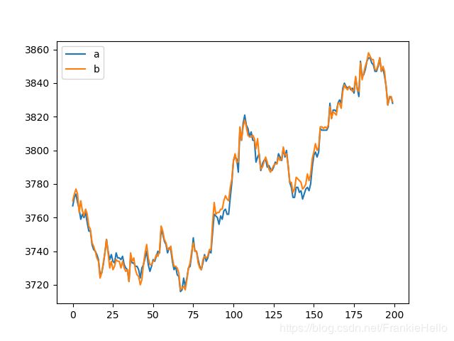
我们从 rb 期货中选择两个品种进行分析，具体的品种根据相关性选择，后期会另外补充。

import numpy as np

import pandas as pd

import matplotlib.pyplot as plt

a_price = pd.read_csv('./CloseA.csv')[:200]

b_price = pd.read_csv('./CloseB.csv')[:200]

fig = plt.figure()

ax = fig.add_subplot(111)

ax.plot(range(len(a_price)), a_price)

ax.plot(range(len(b_price)), b_price)

ax.legend(['a','b'])

plt.show()

从图中看，两个品种具有很强的相关性，并且都是不稳定的。

下面，我们通过ADF检验来看一下，两个序列是否是一阶单整的：

from statsmodels.tsa.stattools import adfuller

a_price = np.reshape(a_price.values, -1)

a_price_diff = np.diff(a_price)

b_price = np.reshape(b_price.values, -1)

b_price_diff = np.diff(b_price)

print(adfuller(a_price_diff))

print(adfuller(b_price_diff))

(-15.436034211511204, 2.90628134201655e-28, 0, 198, {'1%': -3.4638151713286316, '5%': -2.876250632135043, '10%': -2.574611347821651}, 1165.1556545612445)

(-14.259156751414892, 1.4365811614283181e-26, 0, 198, {'1%': -3.4638151713286316, '5%': -2.876250632135043, '10%': -2.574611347821651}, 1152.4222884399824)

从结果来看，两个序列都满足一阶单整，下面来判断两者是否存在协整关系。statsmodels 模块中有 coint函数可以用来检测协整关系，它的内部实现就是基于 EG 协整检验的。

coint 函数如下：

def coint(y0, y1, trend='c', method='aeg', maxlag=None, autolag='aic',

return_results=None):

"""Test for no-cointegration of a univariate equation

The null hypothesis is no cointegration. Variables in y0 and y1 are

assumed to be integrated of order 1, I(1).

This uses the augmented Engle-Granger two-step cointegration test.

Constant or trend is included in 1st stage regression, i.e. in

cointegrating equation.

**Warning:** The autolag default has changed compared to statsmodels 0.8.

In 0.8 autolag was always None, no the keyword is used and defaults to

'aic'. Use `autolag=None` to avoid the lag search.

Parameters

----------

y1 : array_like, 1d

first element in cointegrating vector

y2 : array_like

remaining elements in cointegrating vector

trend : str {'c', 'ct'}

trend term included in regression for cointegrating equation

* 'c' : constant

* 'ct' : constant and linear trend

* also available quadratic trend 'ctt', and no constant 'nc'

method : string

currently only 'aeg' for augmented Engle-Granger test is available.

default might change.

maxlag : None or int

keyword for `adfuller`, largest or given number of lags

autolag : string

keyword for `adfuller`, lag selection criterion.

* if None, then maxlag lags are used without lag search

* if 'AIC' (default) or 'BIC', then the number of lags is chosen

to minimize the corresponding information criterion

* 't-stat' based choice of maxlag.  Starts with maxlag and drops a

lag until the t-statistic on the last lag length is significant

using a 5%-sized test

return_results : bool

for future compatibility, currently only tuple available.

If True, then a results instance is returned. Otherwise, a tuple

with the test outcome is returned.

Set `return_results=False` to avoid future changes in return.

Returns

-------

coint_t : float

t-statistic of unit-root test on residuals

pvalue : float

MacKinnon's approximate, asymptotic p-value based on MacKinnon (1994)

crit_value : dict

Critical values for the test statistic at the 1 %, 5 %, and 10 %

levels based on regression curve. This depends on the number of

observations.

Notes

-----

from statsmodels.tsa.stattools import coint

print(coint(a_price, b_price))

(-3.9532731584015215, 0.008362293067615467, array([-3.95232129, -3.36700631, -3.06583125]))

从返回结果可以看出 t-statistic 值要小于1%的置信度，所以有99%的把握拒绝原假设，而且p-value的值也比较小，所以说存在协整关系。

Ref :

《统计套利：理论与实战》金志宏著

扫一扫，关注我：