十三种基于直方图的图像全局二值化算法原理、实现、代码及效果

1. 什么是基于直方图的图像全局二值化算法

本文的内容来自与十三种基于直方图的图像全局二值化算法原理、实现、代码及效果。本文的中的算法是基于图像的灰度直方图进行阈值分割。
所谓图像的灰度直方图是在将图像进行灰度处理后，计算灰度值的分布。也就是每个灰度值在灰度图像中有多少个点。一般情况下，图像灰度值的取值范围为0~255，所以灰度直方图是一个有256个元素的数组。
阈值分割就是找到一个合适阈值，对灰度图像进行处理。大于阈值的设置为255，小于阈值的设置为0。也可以根据需要设为其他数值。这样处理灰度图像，可以将前景与背景做一个区分。
此方法的关键就是计算阈值。在前面的链接中，介绍了13种方法并提供了C语言实现。本文将这些算法用Python进行了重写。

2. 灰度平均值

灰度平均值是图像总像素值/总像素数：
$总像素值=\sum _{g=0}^{255}g\times h(g)$
$总像素数=\sum _{g=0}^{255}h(g)$
总像素数其实就是图像的宽度X图像的长度，也是图像的大小。

# coding:utf8

import numpy as np
import cv2
from matplotlib import pyplot as plt


def GrayHist(img):
    grayHist = np.zeros(256, dtype=np.uint64)
    for v in range(256):
        grayHist[v] = np.sum(img == v)
    return grayHist


def GetMeanThreshold(H):
    Amount = np.sum(H)
    Gray_Sum = np.sum(H*np.arange(256))
    return int(float(Gray_Sum/Amount))


def GrayThreshold(image, maxval=255):
    g = GrayHist(image)
    thresh = GetMeanThreshold(g)
    threshImage_out = image.copy()
    # 大于阈值的都设置为maxval
    threshImage_out[threshImage_out > thresh] = maxval
    # 小于阈值的都设置为0
    threshImage_out[threshImage_out <= thresh] = 0
    return thresh, threshImage_out


if __name__ == "__main__":

    img = cv2.imread('bird.png')
    img_gray = cv2.cvtColor(img, cv2.COLOR_BGR2GRAY)

    th, img_new = GrayThreshold(img_gray)
    th1, img_new_1 = cv2.threshold(img_gray, 146, 255, cv2.THRESH_BINARY)
    print(th, th1)
    plt.subplot(131), plt.imshow(img_gray, cmap='gray')
    plt.title('Original Image'), plt.xticks([]), plt.yticks([])
    plt.subplot(132), plt.imshow(img_new, cmap='gray')
    plt.title('Image'), plt.xticks([]), plt.yticks([])
    plt.subplot(133), plt.imshow(img_new_1, cmap='gray')
    plt.title('CV2 Image1'), plt.xticks([]), plt.yticks([])
    plt.show()

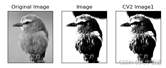
对于小鸟的图像其灰度平均阈值为146。

3. 百分比阈值（P-Tile法）

此方法先设定一个阈值p(先验概率)，比如50%。然后从0开始对灰度值求和。计算到灰度值Y时，[0~Y]的综合>=总像素值*p，则设定灰度值Y为阈值。
该方法需要根据先验概率确定一个百分比。人的经验很重要。

# coding:utf8

import numpy as np
import cv2
from matplotlib import pyplot as plt


def GrayHist(img):
    grayHist = np.zeros(256, dtype=np.uint64)
    for v in range(256):
        grayHist[v] = np.sum(img == v)
    return grayHist


def GetPTileThreshold(H,ptile=0.5):
    Amount = np.sum(H)
    A = Amount * ptile
    psum = 0
    for Y in range(256):
        psum += H[Y]
        if psum >= A:
            return Y
    return -1  # 没有符合条件的阈值


def GrayThreshold(image, maxval=255):
    g = GrayHist(image)
    thresh = GetPTileThreshold(g,0.25)
    threshImage_out = image.copy()
    # 大于阈值的都设置为maxval
    threshImage_out[threshImage_out > thresh] = maxval
    # 小于阈值的都设置为0
    threshImage_out[threshImage_out <= thresh] = 0
    return thresh, threshImage_out


if __name__ == "__main__":

    img = cv2.imread('bird.png')
    img_gray = cv2.cvtColor(img, cv2.COLOR_BGR2GRAY)

    th, img_new = GrayThreshold(img_gray)
    th1, img_new_1 = cv2.threshold(img_gray, 127, 255, cv2.THRESH_BINARY)
    print(th, th1)
    plt.subplot(131), plt.imshow(img_gray, cmap='gray')
    plt.title('Original Image'), plt.xticks([]), plt.yticks([])
    plt.subplot(132), plt.imshow(img_new, cmap='gray')
    plt.title('Image'), plt.xticks([]), plt.yticks([])
    plt.subplot(133), plt.imshow(img_new_1, cmap='gray')
    plt.title('CV2 Image1'), plt.xticks([]), plt.yticks([])
    plt.show()

当百分比设为25%时，阈值为123。这种方法需要认为调节阈值，否则很难得到理想的结果。

3. 基于双峰的阈值

此方法适合与有明显双峰值的图像，对于单峰值或者平坦的灰度直方图形并不适合。
其原理是通过迭代对直方图数据进行判断，判端是否是一个双峰的直方图。如果不是，则对直方图数据进行窗口为3的平滑。如果迭代了一定的数量比如1000次后仍未获得一个双峰的直方图，则函数执行失败。如成功获得，则最终阈值取两个双峰之间的谷底值作为阈值。
所谓窗口为3的平滑，就是将灰度p的值，用p-1，p和p+1的值进行平均。
直方图通过迭代形成双峰后，有2种方法获得阈值：
（1）双峰的平均值
（2）双峰之间的谷底值
第一种方法是找到双峰后，取平均值的整数。第二种方法找到谷底的最小值。

3.1 基于平均值的阈值

# coding:utf8
import numpy as np
import cv2
from matplotlib import pyplot as plt


def GrayHist(img):
    grayHist = np.zeros(256, dtype=np.uint64)
    for v in range(256):
        grayHist[v] = np.sum(img == v)
    return grayHist


def GetIntermodesThreshold(H,method=0):
    Iter = 0
    HistGramC = np.array(H, dtype=np.float64)  # 基于精度问题，一定要用浮点数来处理，否则得不到正确的结果
    HistGramCC = np.array(H, dtype=np.float64)  # 求均值的过程会破坏前面的数据，因此需要两份数据

    # 通过三点求均值来平滑直方图
    while IsDimodal(HistGramCC) == False:  # 判断是否已经是双峰的图像了
        HistGramCC[0] = (HistGramC[0] + HistGramC[0] + HistGramC[1]) / 3  # 第一点
        for Y in range(1, 255):
            HistGramCC[Y] = (HistGramC[Y - 1] + HistGramC[Y] + HistGramC[Y + 1]) / 3  # 中间的点
        HistGramCC[255] = (HistGramC[254] + HistGramC[255] + HistGramC[255]) / 3  # 最后一点
        HistGramC = np.array(HistGramCC, dtype=np.float64)  # 备份数据
        Iter += 1
        if Iter >= 1000:
            return -1  # 直方图无法平滑为双峰的，返回错误代码

    if method > 0:
        Peakfound = False
        for Y in range(1,255):
            if HistGramCC[Y - 1] < HistGramCC[Y] and HistGramCC[Y + 1] < HistGramCC[Y]:
                Peakfound = True
            if Peakfound and HistGramCC[Y - 1] >= HistGramCC[Y] and HistGramCC[Y + 1] >= HistGramCC[Y]:
                return Y - 1
        return -1
    else:
        # 阈值为两峰值的平均值
        Peak = np.zeros(2,dtype=np.uint16)
        Index = 0
        for Y in range(1, 255):
            if HistGramCC[Y - 1] < HistGramCC[Y] and HistGramCC[Y + 1] < HistGramCC[Y]:
                Peak[Index] = Y - 1
                Index += 1
        return int((Peak[0] + Peak[1]) / 2)


def IsDimodal(H):  # 检测直方图是否为双峰的

    # 对直方图的峰进行计数，只有峰数位2才为双峰
    Count = 0
    for Y in range(1, 255):
        if H[Y - 1] < H[Y] and H[Y + 1] < H[Y]:
            Count += 1
            if Count > 2: return False
    if Count == 2:
        return True
    else:
        return False


def GrayThreshold(image, maxval=255):
    g = GrayHist(img_gray)
    thresh = GetIntermodesThreshold(g,1)
    threshImage_out = image.copy()
    # 大于阈值的都设置为maxval
    threshImage_out[threshImage_out > thresh] = maxval
    # 小于阈值的都设置为0
    threshImage_out[threshImage_out <= thresh] = 0
    return thresh, threshImage_out


if __name__ == "__main__":
    img = cv2.imread('bird.png')
    img_gray = cv2.cvtColor(img, cv2.COLOR_BGR2GRAY)

    th1, img_new_1 = cv2.threshold(img_gray, 0, 255, cv2.THRESH_TRIANGLE)
    th, img_new = GrayThreshold(img_gray)
    print(th, th1)
    plt.subplot(131), plt.imshow(img_gray, cmap='gray')
    plt.title('Original Image'), plt.xticks([]), plt.yticks([])
    plt.subplot(132), plt.imshow(img_new, cmap='gray')
    plt.title('Image'), plt.xticks([]), plt.yticks([])
    plt.subplot(133), plt.imshow(img_new_1, cmap='gray')
    plt.title('CV2 Image1'), plt.xticks([]), plt.yticks([])
    plt.show()

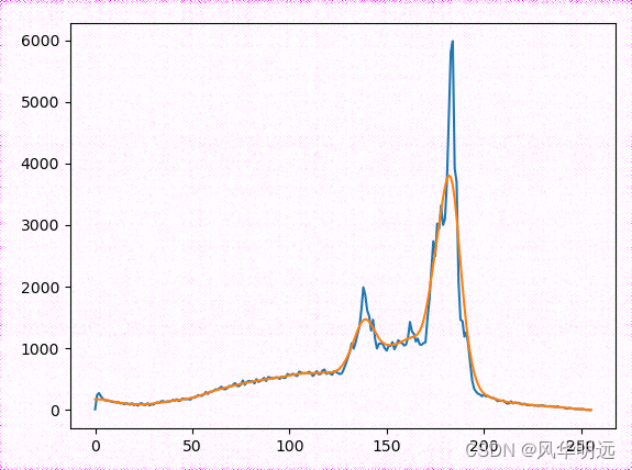
此种方法得到的小鸟图像阈值为159。原始直方图和平滑后的直方图（黄色）如图：

3.2 基于最小值的阈值方法

该方法是查找双峰之间的最小值。使用此方法需要调用GetIntermodesThreshold(g,1)。最后一个参数设置为1即可。

4. 迭代最佳阈值

此方法是先从左边找到HistGram中第一个数值不为0的点min，再从右边找到第一个数值不为0的点max。然后取阈值threshold为此2点的中间值。通过计算[min,threshold]和(threshold,max]平均值灰度值对应的点，进行迭代直到平均灰度值点与阈值点相等。
平均灰度值计算为：
$G_{min}={\sum }_g$