


目录
数据集简介
主要包括3类指标:
- 汽车的各种特性.
- 保险风险评级:(-3, -2, -1, 0, 1, 2, 3).
- 每辆保险车辆年平均相对损失支付.
类别属性
- make: 汽车的商标(奥迪,宝马。。。)
- fuel-type: 汽油还是天然气
- aspiration: 涡轮
- num-of-doors: 两门还是四门
- body-style: 硬顶车、轿车、掀背车、敞篷车
- drive-wheels: 驱动轮
- engine-location: 发动机位置
- engine-type: 发动机类型
- num-of-cylinders: 几个气缸
- fuel-system: 燃油系统
连续指标
- bore: continuous from 2.54 to 3.94.
- stroke: continuous from 2.07 to 4.17.
- compression-ratio: continuous from 7 to 23.
- horsepower: continuous from 48 to 288.
- peak-rpm: continuous from 4150 to 6600.
- city-mpg: continuous from 13 to 49.
- highway-mpg: continuous from 16 to 54.
- price: continuous from 5118 to 45400.
数据的读取与分析
import numpy as np
import pandas as pd
from pandas import datetime

# data visualization and missing values
import matplotlib.pyplot as plt
import seaborn as sns       #Seaborn的底层是基于Matplotlib的,他们的差异有点像在点餐时选套餐还是自己点的区别
import missingno as msno    #missingno提供了一个灵活且易于使用的缺失数据可视化和实用程序的小工具集,使您可以快速直观地总结数据集的完整性。
%matplotlib inline

#stats
from statsmodels.distributions.empirical_distribution import ECDF #它提供对许多不同统计模型估计的类和函数,并且可以进行统计测试和统计数据的探索。
from sklearn.metrics import mean_squared_error,r2_score #机器学习中常用的第三方模块,对常用的机器学习方法进行了封装,包括回归(Regression)、降维(Dimensionality Reduction)、分类(Classfication)、聚类(Clustering)等方法

#mechine learning
from sklearn.preprocessing import StandardScaler
from sklearn.linear_model import Lasso,LassoCV
from sklearn.model_selection import train_test_split,cross_val_score
from sklearn.ensemble import RandomForestRegressor
seed = 123   #切分数据据和交叉验证的时候都会都会有随机策略,制定随机种子后每次随机取数结果都是一样的

data = pd.read_csv("I:/ITLearningMaterials/TYD/MathematicalFoundation/统计分析/回归分析/汽车价格预测/Auto-Data.csv")

data.dtypes
data.describe()  #对于非数值的特征不予统计
缺失值填充
缺失值特性分析
# 分析缺失值
sns.set(style="ticks")
plt.figure(figsize=(12,5))
c = "#366DE8"

#ECDF  经验累积分布函数
plt.subplot(121)
cdf = ECDF(data['normalized-losses'])
plt.plot(cdf.x,cdf.y,label="statmodels",color=c)
plt.xlabel('normalized-losses');plt.ylabel('ECDF')

# 总体分布
plt.subplot(122)
plt.hist(data['normalized-losses'].dropna(),
        bins = int(np.sqrt(len(data['normalized-losses']))),
         color = c)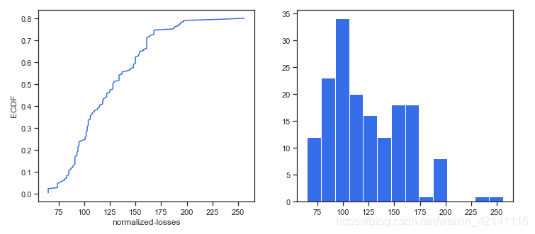
可以看出数据分布不均匀,不适合用平均值填充。大部分情况都可以用中位数填充。但是我们得来想一想,这个特征跟哪些因素可能有关呢?应该是保险的情况吧,所以我们可以分组来进行填充这样会更精确一些。
- 保险风险评级:(-3, -2, -1, 0, 1, 2, 3).
- 每辆保险车辆年平均相对损失支付.
显然是存在关联的。
data.groupby('symboling')['normalized-losses'].describe()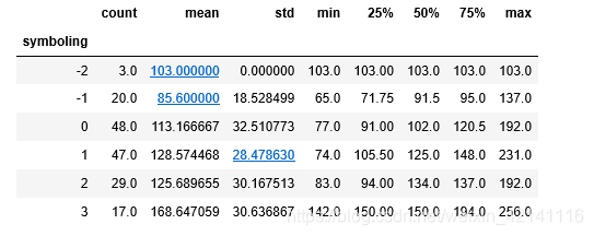
data = data.dropna(subset=['price','bore','stroke','peak-rpm','horsepower','num-of-doors'])  #缺失值较少的列直接剔除缺失项
data['normalized-losses'] = data.groupby('symboling')['normalized-losses'].transform(lambda x:x.fillna(x.mean()))  #填充
关联性分析
cormatrix = data.corr()  #协方差矩阵,协方差表示的是两个变量的总体的误差, 如果两个变量的变化趋势一致,也就是说如果其中一个大于自身的期望值,另外一个也大于自身的期望值,那么两个变量之间的协方差就是正值。
cormatrix *= np.tri(*cormatrix.values.shape,k=-1).T  #返回函数的上三角矩阵,把对角线上的置0,让他们不是最高的。
cormatrix = cormatrix.stack()   #按照类似堆的方式组织数据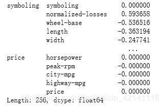
cormatrix = cormatrix.reindex(cormatrix.abs().sort_values(ascending=False).index).reset_index() 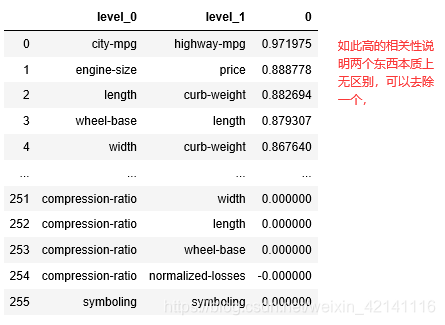
除了剔除相关性过高的以外,还要把有逻辑相关性的剔除部分,比如说汽车生产时候长宽高就有一定的设计比例,如果在我们的统计中还把长宽高作为三个独立的变量就冗余了。
cormatrix.columns = ['FirstVariable','SecondVariable','Corration']  #给列重命名
data['volume'] = data.length*data.width*data.height
data.drop(['width','length','height','curb-weight','city-mpg'],axis=1,inplace=True)
绘制协方差热力图
#计算协方差矩阵
corr_all = data.corr()

#为上三角矩阵制作掩码
mask = np.zeros_like(corr_all,dtype=np.bool)
mask[np.triu_indices_from(mask)] = True

f,ax = plt.subplots(figsize=(11,9))
sns.heatmap(corr_all,mask=mask,square=True,linewidths=.5,ax=ax,cmap="BuPu")
plt.show()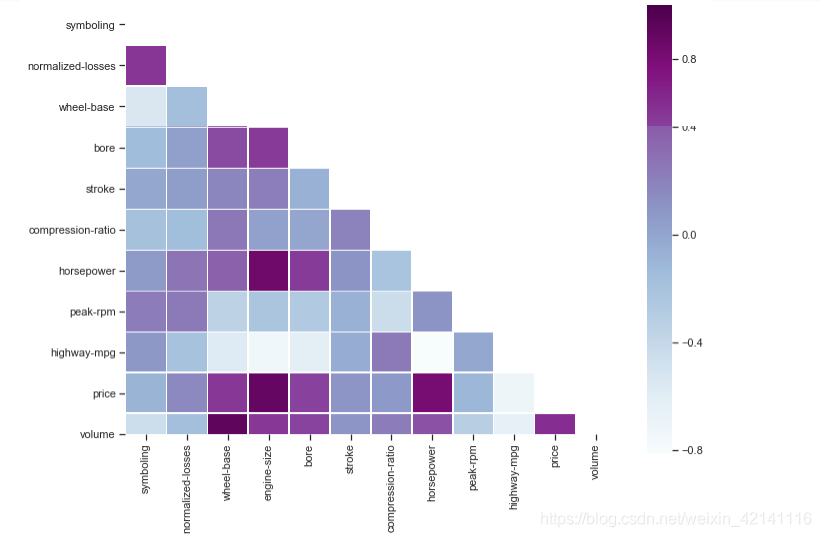
sns.pairplot(data,hue='fuel-type',palette='plasma') #hue指标按照fuel-type来分配颜色,图中两种颜色分别表示燃油和燃气车。palette调色板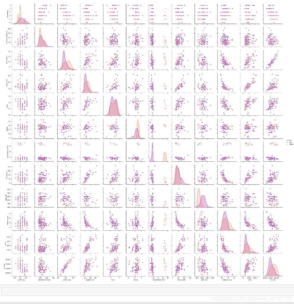
仔细考察价格和马力的关系
sns.lmplot('price','horsepower',data,hue='fuel-type',col='fuel-type',row='num-of-doors',palette='plasma',fit_reg=True)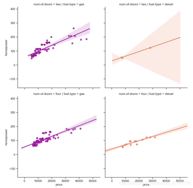
预处理问题
如果一个特性的方差比其他的要大得多,那么它可能支配目标函数,使估计者不能像预期的那样正确地从其他特性中学习。这就是为什么我们需要首先对数据进行缩放。
有些特征的值比较小,比如在0~10之间,有些比较大,比如在100~300之间。这时候会导致我们的数据点集中在坐标轴的某一个特定偏远区域。不利于我们分析,需要将数据调整至坐标轴中央位置。
我们知道,在训练模型的时候,要输入features,即因子,也叫特征。对于同一个特征,不同的样本中的取值可能会相差非常大,一些异常小或异常大的数据会误导模型的正确训练;另外,如果数据的分布很分散也会影响训练结果。以上两种方式都体现在方差会非常大。此时,我们可以将特征中的值进行标准差标准化,即转换为均值为0,方差为1的正态分布。所以在训练模型之前,一定要对特征的数据分布进行探索,并考虑是否有必要将数据进行标准化。
————————————————
版权声明:本文为优快云博主「木子木泗」的原创文章,遵循 CC 4.0 BY-SA 版权协议,转载请附上原文出处链接及本声明。
原文链接:https://blog.youkuaiyun.com/u010758410/article/details/78158781
标准化的流程简单来说可以表达为:将数据按其属性(按列进行)减去其均值,然后除以其方差。最后得到的结果是,对每个属性/每列来说所有数据都聚集在0附近,方差值为1。
基本上拿到手的数据95%以上都需要做标准化
#  对连续值进行标准化
target = data.price

regressors = [x for x in data.columns if x not in ['price']]
features = data.loc[:,regressors]  #以逗号为分隔符,前面的分号表示任何一行,后面的regressors表示指定列
num = ['symboling','normalized-losses','volume','horsepower','wheel-base','bore','stroke','compression-ratio','peak-rpm']

#select the data
standard_scaler = StandardScaler()
features[num] = standard_scaler.fit_transform(features[num])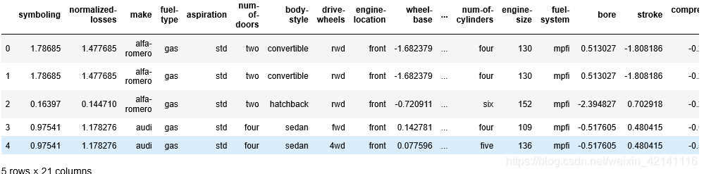
对分类属性进行 one-hot 编码
one-hot编码过程详解
比如:我们要对["中国", "美国", "日本"]进行one-hot编码,
怎么做呢?
1.确定要编码的对象--["中国", "美国", "日本", "美国"],
2.确定分类变量--中国 美国 日本,共3种类别;
3.以上问题就相当于,有3个样本,每个样本有3个特征,将其转化为二进制向量表示,
我们首先进行特征的整数编码:中国--0,美国--1,日本--2,并将特征按照从小到大排列
得到one-hot编码如下

classes = ['make', 'fuel-type', 'aspiration', 'num-of-doors',
           'body-style', 'drive-wheels', 'engine-location',
           'engine-type', 'num-of-cylinders', 'fuel-system']
dummies = pd.get_dummies(features[classes])  #把当前数据全部转换成独立编码
features = features.join(dummies).drop(classes,axis=1)  #连接,替换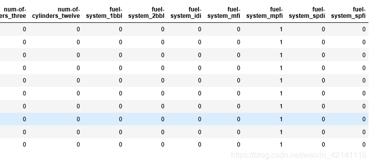
划分训练集与测试集
X_train,X_test,y_train,y_test = train_test_split(features,target,test_size=0.3,random_state=seed)
print(X_test.shape,X_test.shape)   #(58, 66) (58, 66)
回归求解
Lasso回归
多加了一个绝对值项来惩罚过大的系数(强制系数绝对值之和小于某个固定值),alphas=0那就是最小二乘了,alphas越大惩罚力度越大。
# logarithmic scale: log base 2
# high values to zero-out more variables
alphas = 2. ** np.arange(2, 12)  #生成一个一维数组
scores = np.empty_like(alphas)  #empty_like返回一个和输入矩阵shape相同的array

for i, a in enumerate(alphas):   #enumerate() 函数用于将一个可遍历的数据对象(如列表、元组或字符串)组合为一个索引序列,同时列出数据和数据下标,一般用在 for 循环当中。
    lasso = Lasso(random_state = seed)
    lasso.set_params(alpha = a)
    lasso.fit(X_train, y_train)
    scores[i] = lasso.score(X_test, y_test)  #利用测试集获取模型的优劣程度
上面这种方法可以获得比较合适的alpha值,但是不常用(原因不明)
对以上验证做可视化展示
plt.figure(figsize=(10,4))
plt.plot(alphas,scores,'-ko')
plt.axhline(lassocv_score,color='red')
plt.xlabel(r'$\alpha$')
plt.ylabel('CV Score')
plt.xscale('log',basex=2)
sns.despine(offset = 15)     #两根轴的靠近程度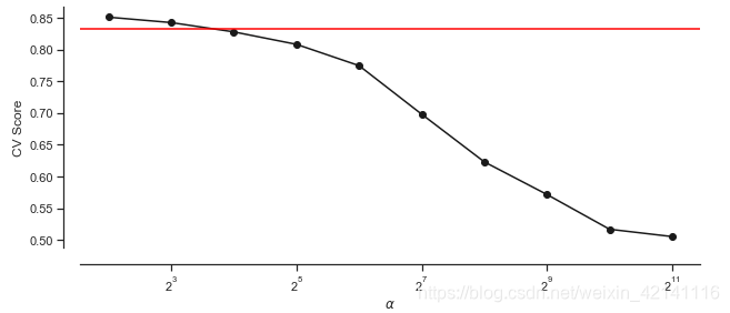
最普遍是做交叉验证:
lassocv = LassoCV(cv = 10, random_state = seed)  #cv交叉验证简称,cv=10,分成十份九份训练一份,
lassocv.fit(features, target)              #features 机器能够识别的数据,target价格列
lassocv_score = lassocv.score(features, target)   #得到score
lassocv_alpha = lassocv.alpha_       #得到score后再把alpha拿出来
检验系数的重要程度,挑选对结果有明显影响的结果
# lassocv coefficients
coefs = pd.Series(lassocv.coef_, index = features.columns)

# prints out the number of picked/eliminated features
print("Lasso picked " + str(sum(coefs != 0)) + " features and eliminated the other " +  \
      str(sum(coefs == 0)) + " features.")

# takes first and last 10
coefs = pd.concat([coefs.sort_values().head(5), coefs.sort_values().tail(5)])

plt.figure(figsize = (10, 4))
coefs.plot(kind = "barh", color = 'red')
plt.title("Coefficients in the Lasso Model")
plt.show()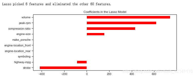
model_l1 = LassoCV(alphas = alphas, cv = 10, random_state = seed).fit(X_train, y_train)
y_pred_l1 = model_l1.predict(X_test)

model_l1.score(X_test, y_test)
0.83307445226244159
We get higher score on the test than on the train set, which shows that the model can propbably generalize well on the unseen data.
绘制残差图
# residual plot
plt.rcParams['figure.figsize'] = (6.0, 6.0)

preds = pd.DataFrame({"preds": model_l1.predict(X_train), "true": y_train})
preds["residuals"] = preds["true"] - preds["preds"]
preds.plot(x = "preds", y = "residuals", kind = "scatter", color = c)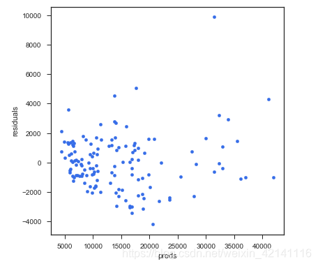
计算MSE和R^2
def MSE(y_true,y_pred):
    mse = mean_squared_error(y_true, y_pred)
    print('MSE: %2.3f' % mse)
    return mse

def R2(y_true,y_pred):
    r2 = r2_score(y_true, y_pred)
    print('R2: %2.3f' % r2)
    return r2

MSE(y_test, y_pred_l1); R2(y_test, y_pred_l1);
MSE: 3870543.789 R2: 0.833
预测
# predictions
d = {'true' : list(y_test),
     'predicted' : pd.Series(y_pred_l1)
    }

pd.DataFrame(d).head()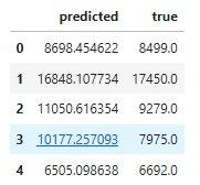


 1296
1296

 被折叠的 条评论
为什么被折叠?
被折叠的 条评论
为什么被折叠?
 到【灌水乐园】发言


