动手学深度学习Task03

第七课 过拟合、欠拟合及其解决方案

验证数据集

作用是对由训练数据集训练出的模型进行选择，比如调参。理由：因为训练误差无法估计泛化误差，因此不该只依赖与训练数据来选择模型。而测试集只能在所有超参数和模型参数选定都使用一次。因此，可以预留出训练集和测试集以外的数据，作为验证数据集。

K折交叉验证

将原始训练数据集划分为K个不重合的子数据集，每次用其中K-1个子数据集进行训练，第K个子数据集进行验证，做K次模型训练和验证。最后，对这K次训练误差和验证误差分别求平均。

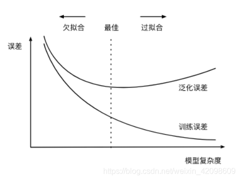
过拟合和欠拟合

欠拟合：模型无法得到较低的训练误差
过拟合：模型在测试集上的误差远远大于在训练集上的误差。
导致两种拟合问题的原因：模型复杂度和数据集大小（原因程度，此两种最常见）。

模型复杂度

模型复杂度和误差之间的关系：

训练数据集大小

影响欠拟合和过拟合的另一个重要因素是训练数据集的大小。一般来说，如果训练数据集中样本数过少，特别是比模型参数数量（按元素计）更少时，过拟合更容易发生。此外，泛化误差不会随训练数据集里样本数量增加而增大。因此，在计算资源允许的范围之内，我们通常希望训练数据集大一些，特别是在模型复杂度较高时，例如层数较多的深度学习模型。

代码理解

1. torch.cat()函数

import torch

# torch.cat((A,B),0) 竖着拼接，即行数增加，列数不变
# torch.cat((A,B),1) 横着拼接，即列数增加，行数不变
x = torch.zeros(2,3)
y = torch.ones(4,3)
z = 2 * torch.ones(2,4)
result1 = torch.cat((x,y),0)
result2 = torch.cat((x,z),1)
print(result1)
print(result2)
output:
tensor([[0., 0., 0.],
        [0., 0., 0.],
        [1., 1., 1.],
        [1., 1., 1.],
        [1., 1., 1.],
        [1., 1., 1.]])
tensor([[0., 0., 0., 2., 2., 2., 2.],
        [0., 0., 0., 2., 2., 2., 2.]])

cat()函数还可以拼接list中的tensor。

2. plt.legend()函数，给图像加上图例，参数以list形式给出。
3. plt.semilogy(x,y)表示x轴为线性刻度，y轴为对数刻度。loglog(x,y)表示x轴和y轴均为对数刻度。

权重衰减

权重衰减等价于$L_2$范数正则化（regularization）。正则化通过为模型损失函数添加惩罚项使学出的模型参数值较小，是应对过拟合的常用手段。
以线性回归损失函数为例：
$$\ell (w_1,w_2,b)=\frac{1}{n}\sum _{i=1}^n\frac{1}{2}{\left(x_1^{(i)}{w}_1+x_2^{(i)}{w}_2+b-y^{(i)}\right)}^2$$

带$L_2$范数惩罚项的损失函数：
$$\ell (w_1,w_2,b)+\frac{\lambda }{2n}|\mathbf{w}{|}^2,$$

因此损失函数在随机梯度下降中，迭代方式变为
$$\begin{array}{rl}{w}_1& \leftarrow \left(1-\frac{\eta \lambda }{|\mathcal{B}|}\right)w_1-\frac{\eta }{|\mathcal{B}|}\sum _{i\in \mathcal{B}}{x}_1^{(i)}\left(x_1^{(i)}{w}_1+x_2^{(i)}{w}_2+b-y^{(i)}\right),\\ w_2& \leftarrow \left(1-\frac{\eta \lambda }{|\mathcal{B}|}\right)w_2-\frac{\eta }{|\mathcal{B}|}\sum _{i\in \mathcal{B}}{x}_2^{(i)}\left(x_1^{(i)}{w}_1+x_2^{(i)}{w}_2+b-y^{(i)}\right).\end{array}$$

可见，$L_2$范数正则化令权重${\omega }_1$和${\omega }_2$先自乘小于1的数，再减去不含惩罚项的梯度。因此，$L_2$范数正则化又叫权重衰减。权重衰减通过惩罚绝对值较大的模型参数为需要学习的模型增加了限制，这可能对过拟合有效。

pytorch实现：

def fit_and_plot_pytorch(wd):
    # 对权重参数衰减。权重名称一般是以weight结尾
    net = nn.Linear(num_inputs, 1)
    nn.init.normal_(net.weight, mean=0, std=1)
    nn.init.normal_(net.bias, mean=0, std=1)
    optimizer_w = torch.optim.SGD(params=[net.weight], lr=lr, weight_decay=wd) # 对权重参数衰减
    optimizer_b = torch.optim.SGD(params=[net.bias], lr=lr)  # 不对偏差参数衰减
    
    train_ls, test_ls = [], []
    for _ in range(num_epochs):
        for X, y in train_iter:
            l = loss(net(X), y).mean()
            optimizer_w.zero_grad()
            optimizer_b.zero_grad()
            
            l.backward()
            
            # 对两个optimizer实例分别调用step函数，从而分别更新权重和偏差
            optimizer_w.step()
            optimizer_b.step()
        train_ls.append(loss(net(train_features), train_labels).mean().item())
        test_ls.append(loss(net(test_features), test_labels).mean().item())
    d2l.semilogy(range(1, num_epochs + 1), train_ls, 'epochs', 'loss',
                 range(1, num_epochs + 1), test_ls, ['train', 'test'])
    print('L2 norm of w:', net.weight.data.norm().item())

优化函数、权重衰减封装在SDG里，只要启用即可。

丢弃法（Dropout）

当对隐藏层使用丢弃法时，该层的隐藏单元将有一定概率被丢弃掉。设丢弃概率为$p$，那么有$p$的概率$h_i$会被清零，有$1-p$的概率会除以$h_i$做拉伸。

def dropout(X, drop_prob):
    X = X.float()
    assert 0 <= drop_prob <= 1
    keep_prob = 1 - drop_prob
    # 这种情况下把全部元素都丢弃
    if keep_prob == 0:
        return torch.zeros_like(X)
    mask = (torch.rand(X.shape) < keep_prob).float()
    
    return mask * X / keep_prob
example:
X = torch.arange(16).view(2, 8)
dropout(X, 0)
tensor([[ 0.,  1.,  2.,  3.,  4.,  5.,  6.,  7.],
        [ 8.,  9., 10., 11., 12., 13., 14., 15.]])
dropout(X, 0.5)
tensor([[ 0.,  0.,  0.,  6.,  8., 10.,  0., 14.],
        [ 0.,  0., 20.,  0.,  0.,  0., 28.,  0.]])
dropout(X, 1.0)
tensor([[0., 0., 0., 0., 0., 0., 0., 0.],
        [0., 0., 0., 0., 0., 0., 0., 0.]])

1. assert函数：断言声明的布尔值必须为真，否则就发生异常。

def evaluate_accuracy(data_iter, net):
    acc_sum, n = 0.0, 0
    for X, y in data_iter:
        if isinstance(net, torch.nn.Module):
            net.eval() # 评估模式, 这会关闭dropout
            acc_sum += (net(X).argmax(dim=1) == y).float().sum().item()
            net.train() # 改回训练模式
        else: # 自定义的模型
            if('is_training' in net.__code__.co_varnames): # 如果有is_training这个参数
                # 将is_training设置成False
                acc_sum += (net(X, is_training=False).argmax(dim=1) == y).float().sum().item() 
            else:
                acc_sum += (net(X).argmax(dim=1) == y).float().sum().item() 
        n += y.shape[0]
    return acc_sum / n

if isinstance(net, torch.nn.Module)判断net是不是nn.Module，是的话直接使用.eval()模式，会关闭dropout。计算完准确率之后，再改回训练模式，如果是自定义模型，就判断是否有is_training参数，如果有，就将此参数改为False，再求准确率，如果没有此参数，直接计算准确率。

第八课 梯度消失、梯度爆炸以及Kaggle房价预测

PyTorch的默认随机初始化

随机初始化模型参数的方法有很多。在线性回归的简洁实现中，我们使用torch.nn.init.normal_()使模型net的权重参数采用正态分布的随机初始化方式。不过，PyTorch中nn.Module的模块参数都采取了较为合理的初始化策略（不同类型的layer具体采样的哪一种初始化方法的可参考源代码），因此一般不用我们考虑。

Xavier随机初始化

还有一种比较常用的随机初始化方法叫作Xavier随机初始化。 假设某全连接层的输入个数为$a$，输出个数为$b$，Xavier随机初始化将使该层中权重参数的每个元素都随机采样于均匀分布
$$U\left(-\sqrt{\frac{6}{a+b}},\sqrt{\frac{6}{a+b}}\right).$$

它的设计主要考虑到，模型参数初始化后，每层输出的方差不该受该层输入个数影响，且每层梯度的方差也不该受该层输出个数影响。具体推到可参考Xavier随机初始化

协变量偏移（不是特别理解）

这里我们假设，虽然输入的分布$P(x)$可能随时间而改变，但是标记函数，即条件分布$P(y\mid x)$不会改变。虽然这个问题容易理解，但在实践中也容易忽视。

想想区分猫和狗的一个例子。我们的训练数据使用的是猫和狗的真实的照片，但是在测试时，我们被要求对猫和狗的卡通图片进行分类。

统计学家称这种协变量变化是因为问题的根源在于特征分布的变化（即协变量的变化）。数学上，我们可以说$P(x)$改变了，但$P(y\mid x)$保持不变。尽管它的有用性并不局限于此，当我们认为x导致y时，协变量移位通常是正确的假设。

标签偏移

当我们认为导致偏移的是标签$P(y)$上的边缘分布的变化，但类条件分布是不变的$P(x\mid y)$时，就会出现相反的问题。当我们认为$y$导致$x$时，标签偏移是一个合理的假设。
病因（要预测的诊断结果）导致 症状（观察到的结果）。
训练数据集，数据很少只包含流感$p(y)$的样本。
而测试数据集有流感$p(y)$和流感$q(y)$，其中不变的是流感症状$p(x|y)$。

概念偏移

另一个相关的问题出现在概念转换中，即标签本身的定义发生变化的情况。

Kaggle房价预测

# 排除类型是object的特征
numeric_features = all_features.dtypes[all_features.dtypes != 'object'].index
all_features[numeric_features] = all_features[numeric_features].apply(
    lambda x: (x - x.mean()) / (x.std()))
# 标准化后，每个数值特征的均值变为0，所以可以直接用0来替换缺失值
all_features[numeric_features] = all_features[numeric_features].fillna(0)

接下来将离散数值转成指示特征。举个例子，假设特征MSZoning里面有两个不同的离散值RL和RM，那么这一步转换将去掉MSZoning特征，并新加两个特征MSZoning_RL和MSZoning_RM，其值为0或1。如果一个样本原来在MSZoning里的值为RL，那么有MSZoning_RL=1且MSZoning_RM=0。这一步操作是利用pd.get_dummies()函数实现的，该函数的具体用法参考get_dummies。

K折交叉验证

   def get_k_fold_data(k, i, X, y):
    # 返回第i折交叉验证时所需要的训练和验证数据
    assert k > 1
    fold_size = X.shape[0] // k
    X_train, y_train = None, None
    for j in range(k):
        idx = slice(j * fold_size, (j + 1) * fold_size)
        X_part, y_part = X[idx, :], y[idx]
        if j == i:
            X_valid, y_valid = X_part, y_part
        elif X_train is None:
            X_train, y_train = X_part, y_part
        else:
            X_train = torch.cat((X_train, X_part), dim=0)
            y_train = torch.cat((y_train, y_part), dim=0)
    return X_train, y_train, X_valid, y_valid

1. slice(start, stop[, step])：实现切片对象，主要用在切片操作函数里的参数传递。start – 起始位置；stop – 结束位置；step – 间距。

第九课 神经网络基础

二维互相关运算实现：
输入数组X与核数组K，输出数组Y。

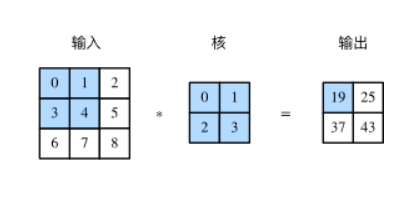
代码实现：

def corr2d(X, K):
    H, W = X.shape
    h, w = K.shape
    Y = torch.zeros(H - h + 1, W - w + 1)
    for i in range(Y.shape[0]):
        for j in range(Y.shape[1]):
            Y[i, j] = (X[i: i + h, j: j + w] * K).sum()
    return Y

二维卷积层的实现：

class Conv2D(nn.Module):
    def __init__(self, kernel_size):
        super(Conv2D, self).__init__()
        self.weight = nn.Parameter(torch.randn(kernel_size))
        self.bias = nn.Parameter(torch.randn(1))

    def forward(self, x):
        return corr2d(x, self.weight) + self.bias

卷积层的简洁实现

我们使用Pytorch中的nn.Conv2d类来实现二维卷积层，主要关注以下几个构造函数参数：

in_channels (python:int) – Number of channels in the input imag
out_channels (python:int) – Number of channels produced by the convolution
kernel_size (python:int or tuple) – Size of the convolving kernel
stride (python:int or tuple, optional) – Stride of the convolution. Default: 1
padding (python:int or tuple, optional) – Zero-padding added to both sides of the input. Default: 0
bias (bool, optional) – If True, adds a learnable bias to the output. Default: True

forward函数的参数为一个四维张量，形状为$(N,C_{in},H_{in},W_{in})$，返回值也是一个四维张量，形状为$(N,C_{out},H_{out},W_{out})$，其中$N$是批量大小，$C,H,W$分别表示通道数、高度、宽度。

池化层

我们使用Pytorch中的nn.MaxPool2d实现最大池化层，关注以下构造函数参数：

kernel_size – the size of the window to take a max over
stride – the stride of the window. Default value is kernel_size
padding – implicit zero padding to be added on both sides