


 本文介绍了ARIMA模型在时间序列预测中的应用,包括模型原理、数据预处理、差分平稳化、ACF和PACF函数的使用来确定p、d、q参数,以及模型的建立、检验和预测。通过AIC、BIC准则选择最优模型,并通过残差检验、D-W检验和Ljung-Box检验确保模型的白噪声性质。最后,展示了模型的预测能力。
ARIMA模型
平稳性:
平稳性就是要求经由样本时间序列所得到的拟合曲线
在未来的一段期间内仍能顺着现有的形态“惯性”地延续下去
平稳性要求序列的均值和方差不发生明显变化
严平稳与弱平稳:
严平稳:严平稳表示的分布不随时间的改变而改变。
弱平稳:期望与相关系数(依赖性)不变
未来某时刻的t的值Xt就要依赖于它过去的信息,所以需要依赖性
1.导包
#美国消费者信心指数
import pandas as pd
import numpy as np
import statsmodels #时间序列
import seaborn as sns
import matplotlib.pylab as plt
from scipy import  stats
import matplotlib.pyplot as plt
2.数据预处理
#1.数据预处理
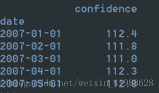
Sentiment = pd.read_csv('confidence.csv', index_col='date', parse_dates=['date'])
#index_col=0, parse_dates=[0]
print(Sentiment.head())
#切分为测试数据和训练数据
n_sample = Sentiment.shape[0]
n_train = int(0.95 * n_sample)+1
n_forecast = n_sample - n_train
ts_train = Sentiment.iloc[:n_train]['confidence']
ts_test = Sentiment.iloc[:n_forecast]['confidence']
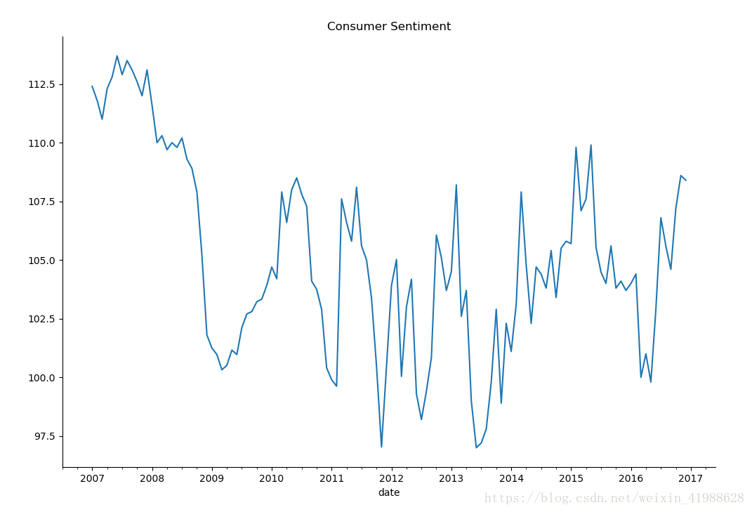
sentiment_short = Sentiment.loc['2007':'2017']
sentiment_short.plot(figsize = (12,8))
plt.title("Consumer Sentiment")
plt.legend(bbox_to_anchor = (1.25,0.5))
sns.despine()
plt.show()结果:注意pandas默认的时间格式是2017-01-01
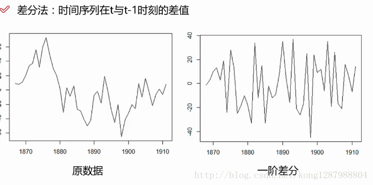
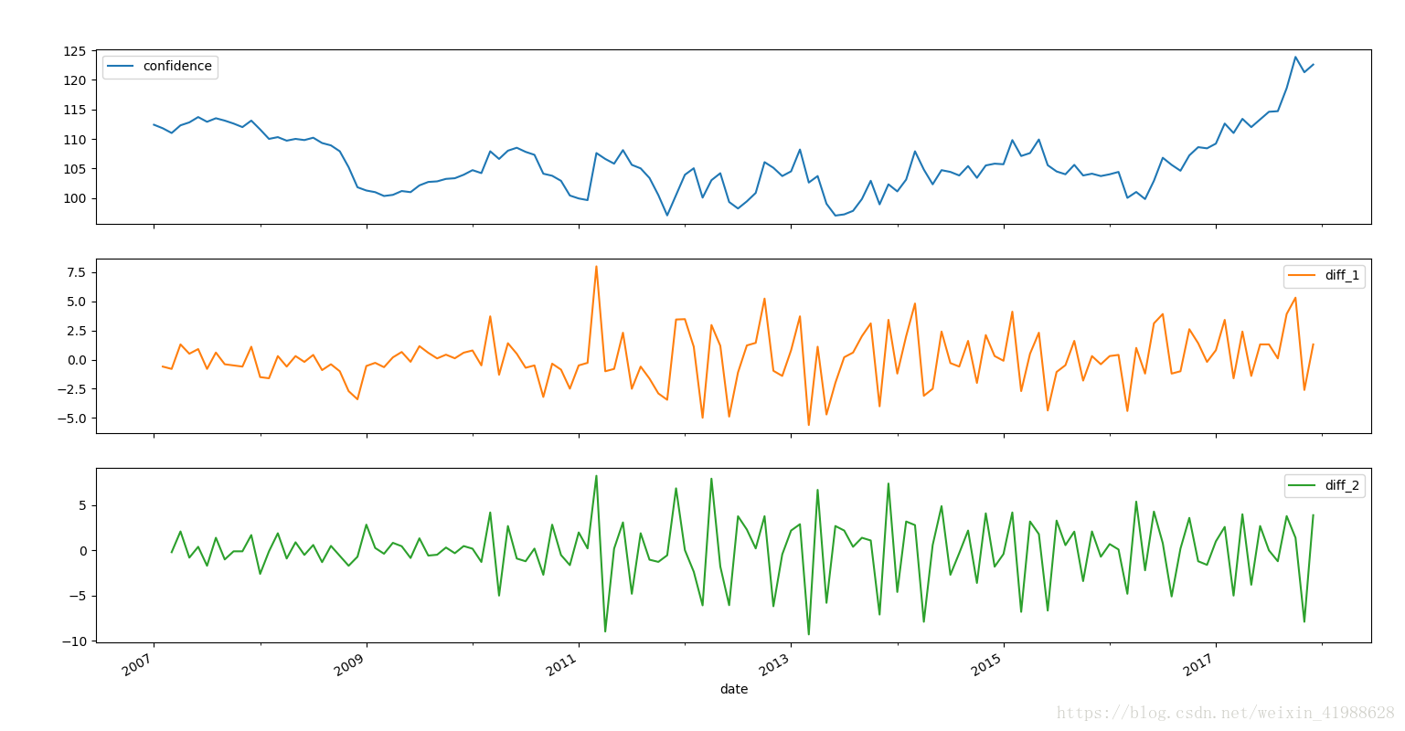
3.时间序列的差分d——将序列平稳化
#2.时间序列的差分d——将序列平稳化
sentiment_short['diff_1'] = sentiment_short['confidence'].diff(1)
# 1个时间间隔,一阶差分,再一次是二阶差分
sentiment_short['diff_2'] = sentiment_short['diff_1'].diff(1)

sentiment_short.plot(subplots=True, figsize=(18, 12))

sentiment_short= sentiment_short.diff(1)


fig = plt.figure(figsize=(12,8))
ax1= fig.add_subplot(111)
diff1 = sentiment_short.diff(1)
diff1.plot(ax=ax1)

fig = plt.figure(figsize=(12,8))
ax2= fig.add_subplot(111)
diff2 = dta.diff(2)
diff2.plot(ax=ax2)

plt.show()
结果:
ARIMA模型原理
自回归模型AR
描述当前值与历史值之间的关系,用变量自身的历史时间数据对自身进行预测
自回归模型必须满足平稳性的要求
p阶自回归过程的公式定义:
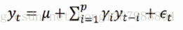
yt是当前值 u是常数项 P是阶数 ri是自相关系数 et是误差
(P当前值距p天前的值的关系)
自回归模型的限制
1、自回归模型是用自身的数据进行预测
2、必
 最低0.47元/天 解锁文章


 3万+
3万+

 被折叠的 条评论
为什么被折叠?
被折叠的 条评论
为什么被折叠?
 到【灌水乐园】发言


