在线销售数据分析–人货场三维分析角度

一、数据来源及理解

此次分析数据来源于第二届Power BI 可视化大赛样例数据，共有四个表，分别为sales
，store，item，district，一共有七十万左右的数据。

二、分析思路

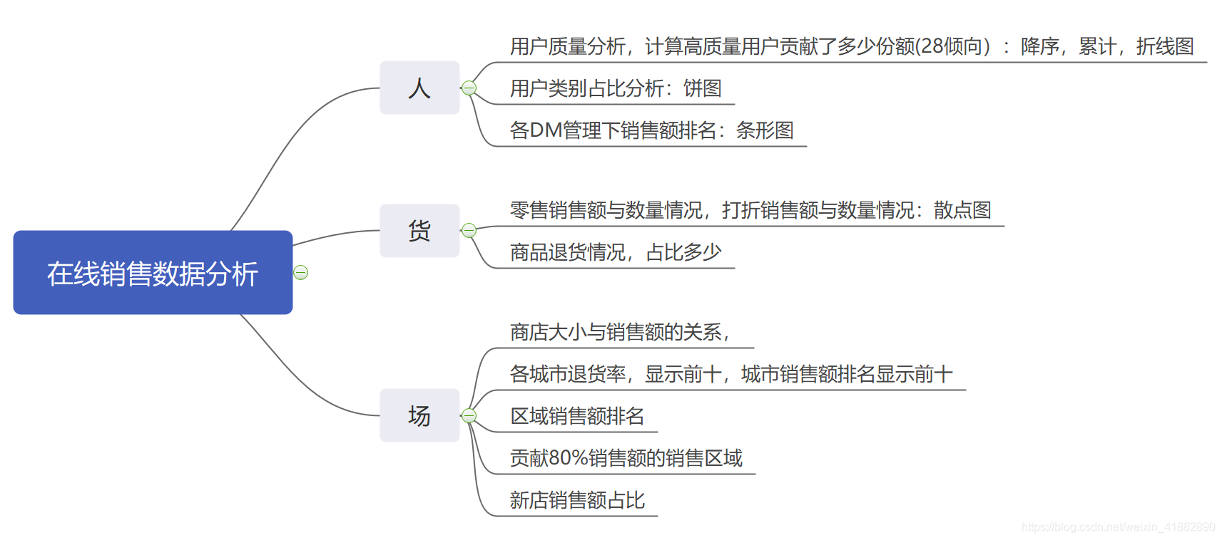
按照人-货-场三维分析角度进行分析，分析导图：

三、数据处理

数据预处理

整个数据包括四张表，三十九个不同字段，但在实际分析过程中我们只用到了十五个字段，为了让数据分析更高效，所以我复制了一份并对其进行一个整合，成为一张表。

数据清洗

利用Python语言进行数据分析，开发工具有Jupyter Notebook，利用的包主要是pandas、numpy，matplotlib.pyplot。

import pandas as pd
import numpy as np
import matplotlib.pyplot as plt
%matplotlib inline
#coding=utf-8
file_name = 'D:\\Analysis.xlsx'
xls = pd.ExcelFile(file_name)
xs = xls.parse('salesdata',dtype='object')
plt.rcParams['font.sans-serif']=['SimHei'] #显示中文
plt.rcParams['axes.unicode_minus']=False #允许显示负数
xs.info()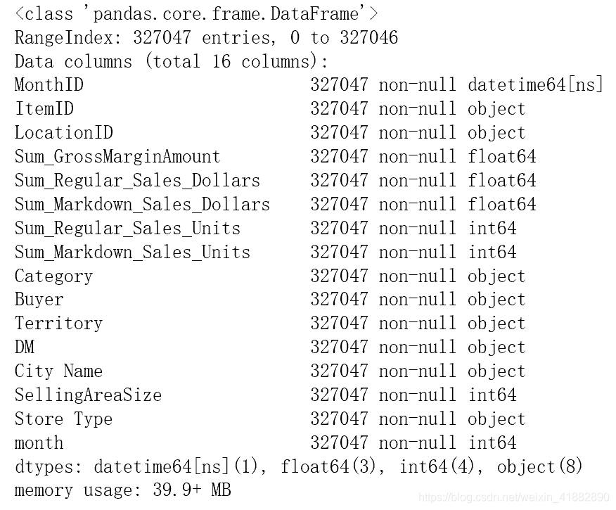

数据总共为327047 条，包含15个特征，接下对数据进行观察并做数据清洗处理。本次数据集比较“干净”，不存在缺失值。另外有些特征的属性需要更改，例如金额及销量的数据类型。

数据转换

数据类型全为object类型，转换数据类型为数值型

xs['Sum_GrossMarginAmount']=pd.to_numeric(xs['Sum_GrossMarginAmount'], errors='coerce').fillna(0) ##数据文本型转换为数值型
xs['Sum_Regular_Sales_Dollars']=pd.to_numeric(xs['Sum_Regular_Sales_Dollars'], errors='coerce').fillna(0)
xs['Sum_Markdown_Sales_Dollars']=pd.to_numeric(xs['Sum_Markdown_Sales_Dollars'], errors='coerce').fillna(0)
xs['Sum_Regular_Sales_Units']=pd.to_numeric(xs['Sum_Regular_Sales_Units'], errors='coerce').fillna(0)
xs['Sum_Markdown_Sales_Units']=pd.to_numeric(xs['Sum_Markdown_Sales_Units'], errors='coerce').fillna(0)
xs['SellingAreaSize']=pd.to_numeric(xs['SellingAreaSize'], errors='coerce').fillna(0)

由于在本次数据集中没有明确的时间字段，所以我们在这不做时间维度的分析，如果要做时间维度的分析还需要对时间字段做一个类型转换。

四、数据描述性统计

xs[['Sum_GrossMarginAmount','Sum_Regular_Sales_Dollars','Sum_Markdown_Sales_Dollars','Sum_Regular_Sales_Units','Sum_Markdown_Sales_Units']].describe()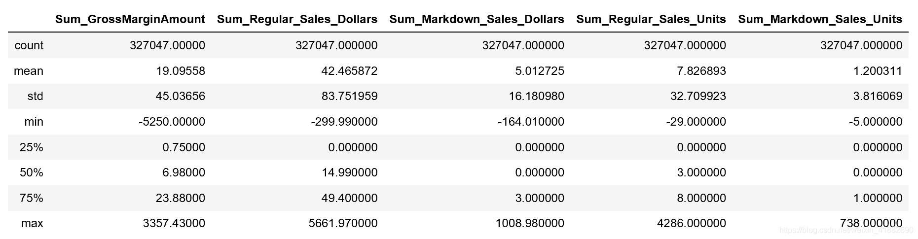

可以看到在销售金额中存在着负数，这可能是退货的订单，需要进行筛选。可以看出各字段的平均值都在百分之75的订单之下，表明存在了一些购买力极强的用户。我们可以将图做出来会更加明显。以’Sum_Regular_Sales_Dollars’字段为例：

plt.subplot(341)
xs['Sum_Regular_Sales_Dollars'].hist(figsize=(10,6),bins=100,color='c')
plt.subplot(342)
xs[xs['Sum_Regular_Sales_Dollars']<1000]['Sum_Regular_Sales_Dollars'].hist(figsize=(10,6),bins=10,color='c')
plt.subplot(343)
xs[xs['Sum_Regular_Sales_Dollars']>3150]['Sum_Regular_Sales_Dollars'].hist(figsize=(10