Regression with scikit-learn

Regression with scikit-learn

Fit & predict for regression

# Import LinearRegression
from sklearn.linear_model import LinearRegression

# Create the regressor: reg
reg = LinearRegression()

# Create the prediction space
prediction_space = np.linspace(min(X_fertility), max(X_fertility)).reshape(-1,1)

# Fit the model to the data
reg.fit(X_fertility, y)

# Compute predictions over the prediction space: y_pred
y_pred = reg.predict(prediction_space)

# Print R^2 
print(reg.score(X_fertility, y))

# Plot regression line
plt.plot(prediction_space, y_pred, color='black', linewidth=3)
plt.show()

Train/test split for regression

# Import necessary modules
from sklearn.linear_model import LinearRegression
from sklearn.metrics import mean_squared_error
from sklearn.model_selection import train_test_split

# Create training and test sets
X_train, X_test, y_train, y_test = train_test_split(X, y, test_size = 0.3, random_state=42)

# Create the regressor: reg_all
reg_all = LinearRegression()

# Fit the regressor to the training data
reg_all.fit(X_train, y_train)

# Predict on the test data: y_pred
y_pred = reg_all.predict(X_test)

# Compute and print R^2 and RMSE
print("R^2: {}".format(reg_all.score(X_test, y_test)))
rmse = np.sqrt(mean_squared_error(y_test, y_pred))
print("Root Mean Squared Error: {}".format(rmse))

5-fold cross-validation

# Import the necessary modules
from sklearn.linear_model import LinearRegression
from sklearn.model_selection import cross_val_score

# Create a linear regression object: reg
reg = LinearRegression()

# Compute 5-fold cross-validation scores: cv_scores
cv_scores = cross_val_score(reg, X, y, cv=5)

# Print the 5-fold cross-validation scores
print(cv_scores)

# Print the average 5-fold cross-validation score
print("Average 5-Fold CV Score: {}".format(np.mean(cv_scores)))

K-Fold CV comparison

# Import necessary modules
from sklearn.linear_model import LinearRegression
from sklearn.model_selection import cross_val_score

# Create a linear regression object: reg
reg = LinearRegression()

# Perform 3-fold CV
cvscores_3 = cross_val_score(reg, X, y, cv = 3)
print(np.mean(cvscores_3))

# Perform 10-fold CV
cvscores_10 = cross_val_score(reg, X, y, cv = 10)
print(np.mean(cvscores_10))

Regularized regression

why regularize?
It chooses a coefficient for each feature variable.
Large coefficients can lead to overfitting
Penalizing large coefficients:Regularization.

Regularization I: Lasso

# Import Lasso
from sklearn.linear_model import Lasso

# Instantiate a lasso regressor: lasso
lasso = Lasso(alpha=0.4, normalize=True)

# Fit the regressor to the data
lasso.fit(X, y)

# Compute and print the coefficients
lasso_coef = lasso.coef_
print(lasso_coef)

# Plot the coefficients
plt.plot(range(len(df_columns)), lasso_coef)
plt.xticks(range(len(df_columns)), df_columns.values, rotation=60)
plt.margins(0.02)
plt.show()

According to the lasso algorithm, it seems like ‘child_mortality’ is the most important feature when predicting life expectancy.

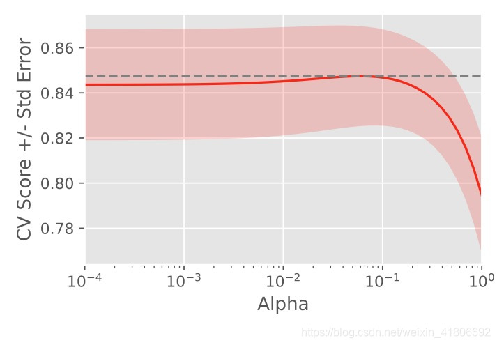
Regularization II: Ridge

Lasso is great for feature selection, but when building regression models, Ridge regression should be your first choice.

# Import necessary modules
from sklearn.linear_model import Ridge
from sklearn.model_selection import cross_val_score

# Setup the array of alphas and lists to store scores
alpha_space = np.logspace(-4, 0, 50)
ridge_scores = []
ridge_scores_std = []

# Create a ridge regressor: ridge
ridge = Ridge(normalize=True)

# Compute scores over range of alphas
for alpha in alpha_space:

    # Specify the alpha value to use: ridge.alpha
    ridge.alpha = alpha
    
    # Perform 10-fold CV: ridge_cv_scores
    ridge_cv_scores = cross_val_score(ridge, X, y, cv=10)
    
    # Append the mean of ridge_cv_scores to ridge_scores
    ridge_scores.append(np.mean(ridge_cv_scores))
    
    # Append the std of ridge_cv_scores to ridge_scores_std
    ridge_scores_std.append(np.std(ridge_cv_scores))

# Display the plot
display_plot(ridge_scores, ridge_scores_std)

Building a logistic regression model

# Import the necessary modules
from sklearn.linear_model import LogisticRegression
from sklearn.metrics import confusion_matrix, classification_report

# Create training and test sets
X_train, X_test, y_train, y_test = train_test_split(X, y, test_size = 0.4, random_state=42)

# Create the classifier: logreg
logreg = LogisticRegression()

# Fit the classifier to the training data
logreg.fit(X_train, y_train)

# Predict the labels of the test set: y_pred
y_pred = logreg.predict(X_test)

# Compute and print the confusion matrix and classification report
print(confusion_matrix(y_test, y_pred))
print(classification_report(y_test, y_pred))

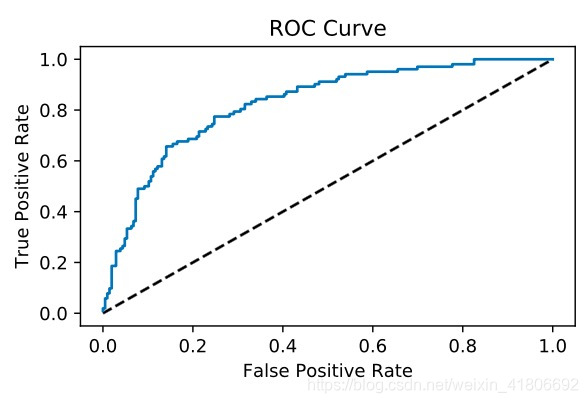
Plotting an ROC curve

# Import necessary modules
from sklearn.metrics import roc_curve

# Compute predicted probabilities: y_pred_prob
y_pred_prob = logreg.predict_proba(X_test)[:,1]

# Generate ROC curve values: fpr, tpr, thresholds
fpr, tpr, thresholds = roc_curve(y_test, y_pred_prob)

# Plot ROC curve
plt.plot([0, 1], [0, 1], 'k--')
plt.plot(fpr, tpr)
plt.xlabel('False Positive Rate')
plt.ylabel('True Positive Rate')
plt.title('ROC Curve')
plt.show()