CV - Detailed Guide to Understand ResNets

今天被男朋友鄙视，因为我说不出来Resnet…(反正他也不看我博客) 哼 本宫这样就把它补上！

Background

Researchers observed that it makes sense to affirm that “the deeper the better” when it comes to convolutional neural networks. This makes sense, since the models should be more capable (their flexibility to adapt to any space increase because they have a bigger parameter space to explore). However, it has been noticed that after some depth, the performance degrades.
This was one of the bottlenecks of VGG. They couldn’t go as deep as wanted.

Architecture

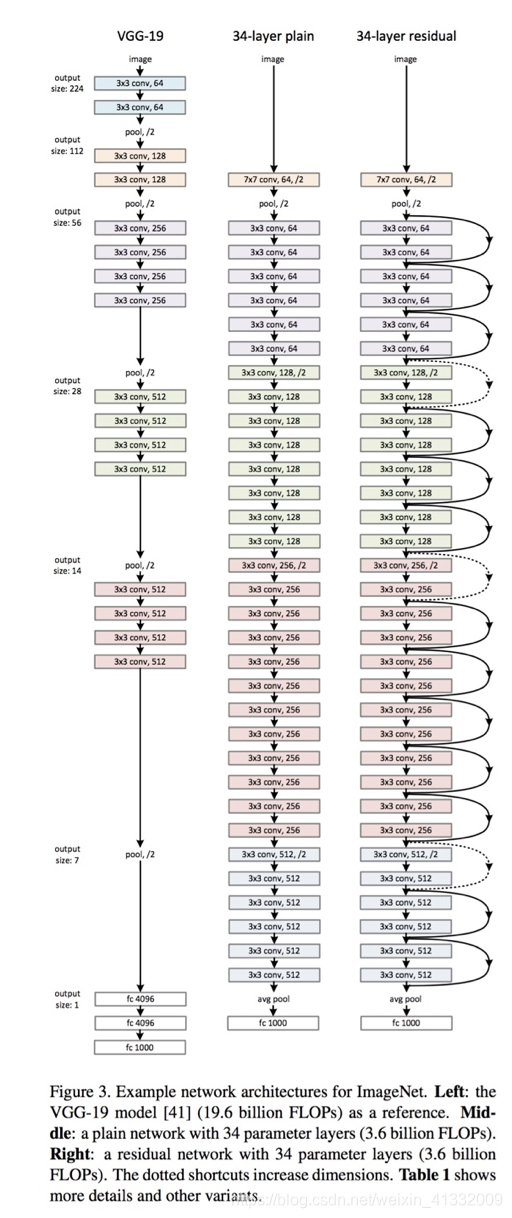
Since ResNets can have variable sizes, depending on how big each of the layers of the model are, and how many layers it has, we will follow the described by the authors in the paper – ResNet 34(which means there are 34 layers)-- in order to explain the structure after these networks.

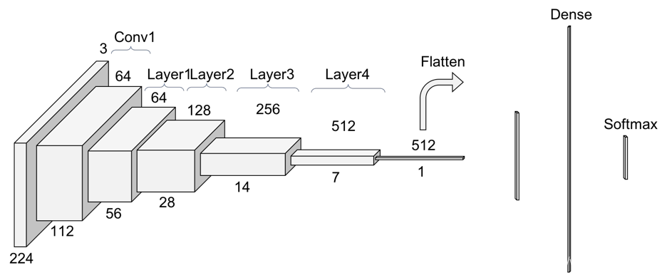
In here we can see that the ResNet (the one on the right) consists one convolution and pooling step (orange) followed by 4 layers of similar behavior.

Each of the layers follow the same pattern. They perform 3x3 convolution with a fixed feature map dimension , i.e. 64, 128, 256, and 512 respectively, bypassing the input every 2 convolutions. Furthermore, the width (W) and height (H) dimensions remain constant during each layer.

let’s go layer by layer!

1. Convolution 1

The first step on the ResNet before entering the common layer behavior is a block — called here Conv1 — consisting on a convolution(kernel:7, out_channel:64) + batch normalization + max pooling operation.

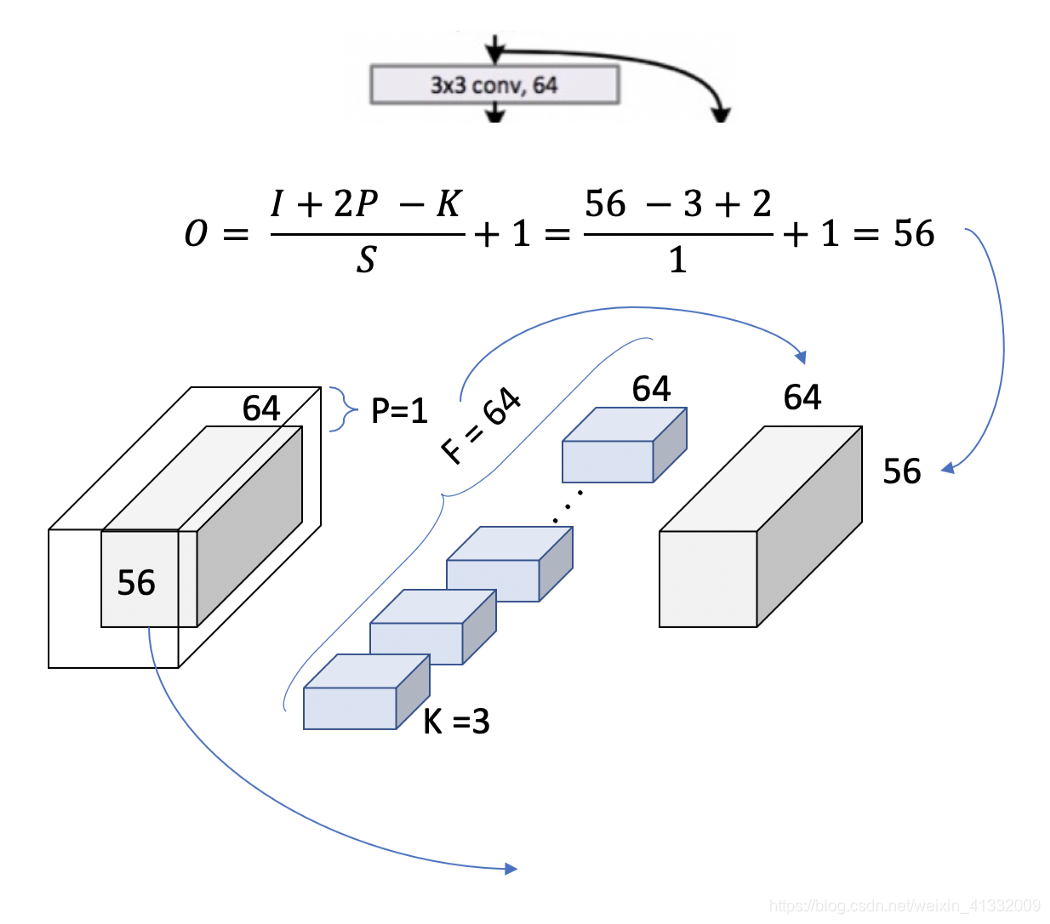
Now let’s look at how exactly does convolution works in the first layer:

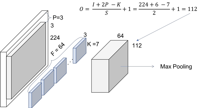
They use a kernel size of 7, and 64 channels(so there will be 64 feature maps), with stride of 2. You need to infer that they have padded with zeros 3 times on each dimension. Therefore, the output size of that operation will be a (112x112) volume. Since each convolution filter (of the 64) is providing one channel in the output volume, we end up with a (112x112x64) output volume.

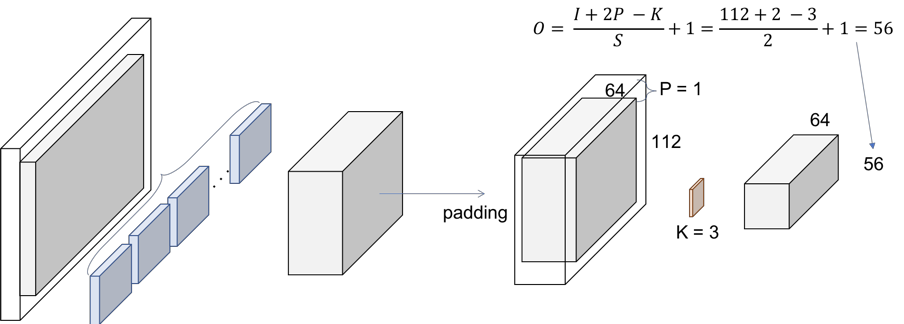
The next step is the batch normalization, which is an element-wise operation and therefore, it does not change the size of our volume. Finally, we have the (3x3) Max Pooling operation with a stride of 2. We can also infer that they first pad the input volume, so the final volume has the desired dimensions.

2. ResNet Layers

So, let’s explain this repeating name, block. Every layer of a ResNet is composed of several blocks. This is because when ResNets go deeper, they normally do it by increasing the number of operations within a block, but the number of total layers remains the same — An operation here refers to a convolution+a batch normalization+and a ReLU activation to an input, except the last operation of a block, that does not have the ReLU.

for a single layer 3*3 conv, 64, the output size is [56x56]

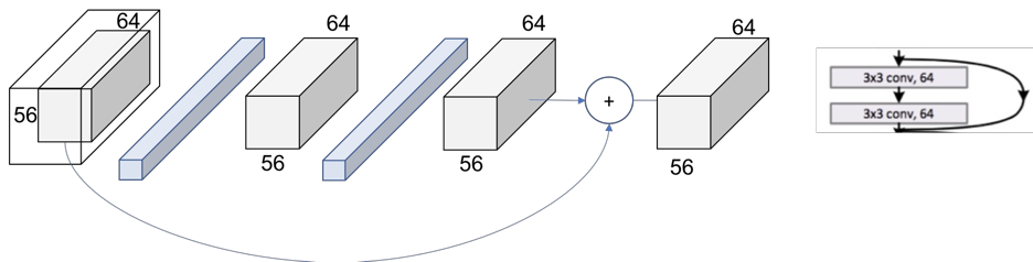
in a residual block, we add skip-connection, and two conv layers:

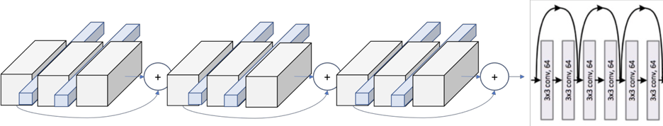
we have the [3x3, 64] x 3 times within the layer

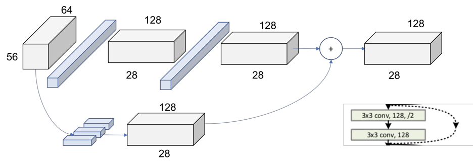
between layers

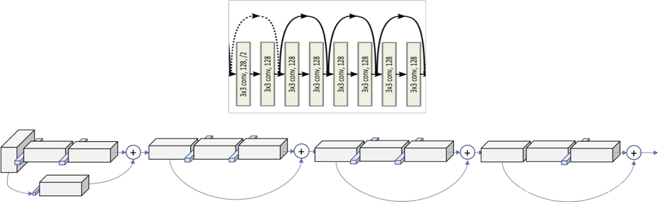
In the Figure 1 we can see how the layers are differentiable by colors. However, if we look at the first operation of each layer, we see that the stride used at that first one is 2, instead of 1 like for the rest of them.

This means that the down sampling of the network is achieved by increasing the stride instead of a pooling operation like normally CNNs do. In fact, only one max pooling operation is performed in our Conv1 layer, and one average pooling layer at the end of the ResNet, right before the fully connected dense layer.

The dot line represents the change of the dimensionality, and the solid line represents BN+RELU

The global picture of a whole layer:

👨‍🏫 Interview Questions for RESNET:

(1) 问题的提出

网络层数增多一般会伴着下面几个问题:

1. 计算资源的消耗。（问题1可以通过GPU集群来解决）
2. 模型容易过拟合。 （问题2的过拟合通过采集海量数据，并配合Dropout正则化等方法也可以有效避免）
3. 梯度消失/梯度爆炸问题的产生。 （问题3通过正则化初始化和中间的Batch Normalization 层可以有效解决）

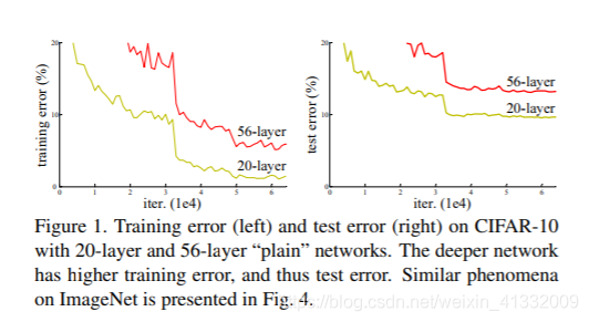
貌似我们只要无脑的增加网络的层数，我们就能从此获益，但实验数据给了我们当头一棒。

作者发现，随着网络层数的增加，网络发生了退化（degradation）的现象：随着网络层数的增多，训练集loss逐渐下降，然后趋于饱和，当你再增加网络深度的话，训练集loss反而会增大。注意这并不是过拟合，因为在过拟合中训练loss是一直减小的。

（2）残差块的作用

• 只做恒等映射也不该出现退化问题
  深度网络的退化问题至少说明深度网络不容易训练。但是考虑以下事实：现在已经有了一个浅层神经网络，通过向上堆积新层来建立深层网络。一个极端情况是这些增加的层什么也不学习，仅仅复制浅层网络的特征，即向上堆积的层仅仅是在做恒等映射（Identity mapping）。在这种情况下，深层网络应该至少和浅层网络性能一样，也不应该出现退化现象。
• 恒等映射不是想学就能学
  但是问题可能是，网络并不是那么容易的就能学到恒等映射。随着网络层数不断加深，求解器不能找到解决途径。

ResNet 就是通过显式的修改网络结构，加入残差通路，让网络更容易的学习到恒等映射。通过改进，我们发现深层神经网络的性能不仅不比浅层神经网络差，还要高出不少。

Plain Net：

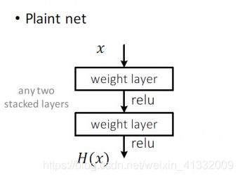
图中的 H(x)代表的是我们最终想要得到的一个映射。在 Plaint net 中，我们就是希望这两层网络能够直接拟合出 H(x)。

Residual Net：

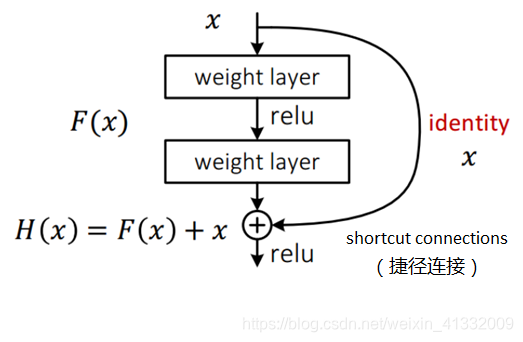
图中的 H(x)代表的仍然是我们最终想要得到的一个映射。与 Plain net 不同的是，这里通过一个捷径连接（shortcut connections）直接将x传到了后面与这两层网络拟合出的结果相加，H(x)是我们最终想要得到的一个映射，假设这两层网络拟合出来的映射为 F(x)，那么 F(x)应该等于 H(x)−x。

做这种变换的作用：
如果 x 已经是最优的了，也就是说我们希望得到的映射 H(x)恰好就是此时的输入x，也就是说要做恒等映射，这个时候只需要将权重值设定为 0。也就是让 F(x)=0就好了。我们发现这比直接学习 H(x)=x要容易的多。

实际上残差网络相当于将学习目标改变了，学习的不再是一个完整的输出，而是目标值 H(x)和 x 的差值，也就是这篇文章一直在讨论的残差 F(x)。并且有 F(x)=H(x)−x。

（3）两种残差学习单元

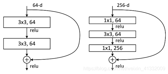
两种结构分别针对ResNet34（左图）和 ResNet50/101/152（右图）。右图的主要目的是减少参数数量。

为了做个详细的对比，我们这里假设左图的残差单元的输入不是 64-d 的，而是 256-d 的，那么左图应该为两个 3×3,256的卷积。参数总数为：$3\times 3\times 256\times 256\times 2=1179648$。对上式做个说明：3×3×256 计算的是每个 filter 的参数数目，第 2 个 256 是说每层有 256 个filter，最后一个 2 是说一共有两层。

右图的输入同样为 256-d 的，首先通过一个 1×1,64
的卷积层将通道数降为 64。然后是一个 3×3,64的卷积层。最后再通过一个 1×1,256的卷积层通道数恢复为 256。参数总数为：$$1\times 1\times 256\times 64+3\times 3\times 64\times 64+1\times 1\times 64\times 256=69632$$
可见参数数量明显变少了。

通常来说对于常规的ResNet，可以用于34层或者更少的网络中（左图）；对于更深的网络（如101层），则使用右图，其目的是减少计算和参数量。

男朋友的补充总结：
Resnet的好处主要体现在
[1] 由于直接将原图x经由恒等变换加到卷积之后的F(x)上，给予下一层的模型不同尺度的信息(类似multi-scale GAN)
[2] 增加了skip-connection，能够让梯度直接传播过去而不用经过梯度bottleneck，缓解了梯度消失问题。
[3] 解决了网络层数越多，网络越退化的问题