线性回归

线性回归模型与诊断

数据说明：本数据是一份汽车贷款数据

字段名	中文含义
id	id
Acc	是否开卡(1=已开通)
avg_exp	月均信用卡支出（元）
avg_exp_ln	月均信用卡支出的自然对数
gender	性别(男=1)
Age	年龄
Income	年收入（万元）
Ownrent	是否自有住房（有=1；无=0)
Selfempl	是否自谋职业(1=yes, 0=no)
dist_home_val	所住小区房屋均价(万元)
dist_avg_income	当地人均收入
high_avg	高出当地平均收入
edu_class	教育等级：小学及以下开通=0，中学=1，本科=2，研究生=3

%matplotlib inline

import matplotlib.pyplot as plt
import os
import numpy as np
import pandas as pd
import statsmodels.api as sm
from statsmodels.formula.api import ols

os.chdir('E:/data')
pd.set_option('display.max_columns', 8)

E:\Anaconda3\lib\site-packages\statsmodels\compat\pandas.py:56: FutureWarning: The pandas.core.datetools module is deprecated and will be removed in a future version. Please use the pandas.tseries module instead.
  from pandas.core import datetools

导入数据和数据清洗

raw = pd.read_csv('creditcard_exp.csv', skipinitialspace=True)
raw.head()

	id	Acc	avg_exp	avg_exp_ln	...	dist_avg_income	age2	high_avg	edu_class
0	19	1	1217.03	7.104169	...	15.932789	1600	0.102361	3
1	5	1	1251.50	7.132098	...	15.796316	1024	0.051184	2
2	95	0	NaN	NaN	...	7.490000	1296	0.910000	1
3	86	1	856.57	6.752936	...	11.275632	1681	0.197218	3
4	50	1	1321.83	7.186772	...	13.346474	784	0.062676	2

5 rows × 14 columns

exp = raw[raw['avg_exp'].notnull()].copy().iloc[:, 2:]\
.drop('age2',axis=1)

exp_new = raw[raw['avg_exp'].isnull()].copy().iloc[:, 2:]\
.drop('age2',axis=1)

exp.describe(include='all')

	avg_exp	avg_exp_ln	gender	Age	...	dist_home_val	dist_avg_income	high_avg	edu_class
count	70.000000	70.000000	70.000000	70.000000	...	70.000000	70.000000	70.000000	70.000000
mean	983.655429	6.787787	0.285714	31.157143	...	74.540857	8.005472	-0.580766	1.928571
std	446.294237	0.476035	0.455016	7.206349	...	36.949228	3.070744	0.432808	0.873464
min	163.180000	5.094854	0.000000	20.000000	...	13.130000	3.828842	-1.526850	0.000000
25%	697.155000	6.547003	0.000000	26.000000	...	49.302500	5.915553	-0.887981	1.000000
50%	884.150000	6.784627	0.000000	30.000000	...	65.660000	7.084184	-0.612068	2.000000
75%	1229.585000	7.114415	1.000000	36.000000	...	105.067500	9.123105	-0.302082	3.000000
max	2430.030000	7.795659	1.000000	55.000000	...	157.900000	18.427000	0.259337	3.000000

8 rows × 11 columns

相关性分析

散点图

exp.plot('Income', 'avg_exp', kind='scatter')
plt.show()

[外链图片转存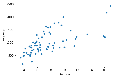(img-0SGvSTVL-1562725477539)(output_7_0.png)]

exp[['Income', 'avg_exp', 'Age', 'dist_home_val']].corr(method='pearson')

	Income	avg_exp	Age	dist_home_val
Income	1.000000	0.674011	0.369129	0.249153
avg_exp	0.674011	1.000000	0.258478	0.319499
Age	0.369129	0.258478	1.000000	0.109323
dist_home_val	0.249153	0.319499	0.109323	1.000000

线性回归算法

简单线性回归

lm_s = ols('avg_exp ~ Income', data=exp).fit()
print(lm_s.params)

Intercept    258.049498
Income        97.728578
dtype: float64

Predict-在原始数据集上得到预测值和残差

lm_s.summary()

OLS Regression Results

Dep. Variable:	avg_exp	R-squared:	0.454
Model:	OLS	Adj. R-squared:	0.446
Method:	Least Squares	F-statistic:	56.61
Date:	Mon, 30 Apr 2018	Prob (F-statistic):	1.60e-10
Time:	16:59:33	Log-Likelihood:	-504.69
No. Observations:	70	AIC:	1013.
Df Residuals:	68	BIC:	1018.
Df Model:	1
Covariance Type:	nonrobust

	coef	std err	t	P>|t|	[0.025	0.975]
Intercept	258.0495	104.290	2.474	0.016	49.942	466.157
Income	97.7286	12.989	7.524	0.000	71.809	123.648

Omnibus:	3.714	Durbin-Watson:	1.424
Prob(Omnibus):	0.156	Jarque-Bera (JB):	3.507
Skew:	0.485	Prob(JB):	0.173
Kurtosis:	2.490	Cond. No.	21.4

pd.DataFrame([lm_s.predict(exp), lm_s.resid], index=['predict', 'resid']
            ).T.head()

	predict	resid
0	1825.141904	-608.111904
1	1806.803136	-555.303136
3	1379.274813	-522.704813
4	1568.506658	-246.676658
5	1238.281793	-422.251793

在待预测数据集上得到预测值

lm_s.predict(exp_new)[:5]

2     1078.969552
11     756.465245
13     736.919530
19     687.077955
20     666.554953
dtype: float64

多元线性回归

lm_m = ols(