2022.05.23 - 2022.05.29

传送门

2022-05-23

Proof of Theorem 1

这个定理假设在向模型中注入 $\Delta$ 后，我们就有了
$$\forall x\in \mathcal{X},Pr({\mathcal{F}}_{\theta }(x+\Delta )=y_t\ne {\mathcal{F}}_{\theta }(x))\ge 1-\mu \text{\hspace{1em}(1)}$$
当攻击者应用基于梯度的优化来寻找对 $y_t$ 的输入 $x$ 的对抗性扰动时，上述方程意味着从 $x$ 到 $x+\Delta$ 的部分梯度成为实现目标 $y_t$ 的主要梯度。注意 ${\mathcal{F}}_{\theta }(x)$ 是非线性特征 $g(x)$ 和线性损失函数（例如逻辑回归) 组成: ${\mathcal{F}}_{\theta }(x)=g(x)\circ L$, 其中 $L$ 表示线性函数。 因此，${\mathcal{F}}_{\theta }(x)$ 的梯度可以通过 $g(x)$ 计算：
$$\frac{\partial \ln {\mathcal{F}}_{\theta }(x)}{\partial x}=\frac{\partial \ln [g(x)\circ L]}{\partial x}=c\frac{\partial \ln g(x)\circ L}{\partial x},\text{\hspace{1em}(2)}$$
其中 $c$ 是线性函数 $L$ 中的常数。为避免歧义，我们将在其余证明中关注 $g(x)$ 的导数。根据公式 $(2)$ , 我们从主要梯度来解释公式 $(1)$:
$$P_{x\in \mathcal{X}}[\frac{\partial [\ln g(x)-\ln g(x+\Delta )]}{\partial x}\ge \eta ]\ge 1-\mu ,\text{\hspace{1em}(3)}$$
其中 $\eta$ 代表把 $x$ 错误分类为 $y_t$ 所需的梯度值。
  因为 $\forall x\in \mathcal{X},cos(g(A(x)),g(x+\Delta ))\ge \sigma$, 其中 $\sigma \to 1$，因此，我们有 $g(A(x))=g(x+\Delta )+\gamma$ 其中 $|\gamma |<<|g(x+\Delta )|$。通过以上条件，我们可以证明下面两个条件。
第一个，因为 $\gamma$ 的值与 $x$ 无关， 我们有
$$\frac{\partial (g(x+\Delta )+\gamma )}{\partial x}=\frac{\partial g(x+\Delta )}{\partial x}\text{\hspace{1em}(4)}$$
第二，因为 $|\gamma |<<|g(x+\Delta )|$ , 有
$$\frac{1}{g(x+\Delta )+\gamma }\approx \frac{1}{g(x+\Delta )}\text{\hspace{1em}(5)}$$
利用公式 $(3)$-$(5)$, 有如下的证明过程

  定理 1 表明 trapdoor 模型将允许攻击者使用任何输入 $x$ 对 $y_t$ 发起非常成功的攻击。更重要的是，相应的对抗性输入 $A(x)$ 将显示特定模式，即其特征表示将类似于 trapdoor 的输入。因此，通过记录 $\Delta$ 的 “trapdoor特征”，即 ${\mathcal{S}}_{\Delta }={\mathbf{E}}_{x\in \mathcal{X},y_t\ne {\mathcal{F}}_{\theta }(x)}g(x+\Delta ),$ 我们可以通过比较它的特征表示和 ${\mathcal{S}}_{\Delta }$来确定模型输入是否是对抗性的。

Case 2: Practical Trapdoor Injection. 到目前为止，我们的分析认为 trapdoor “完美” 地注入了模型。在实践中，模型所有者将用于注入 $\Delta$ 的训练数据定义为 ${\mathcal{X}}_{trap}\in \mathcal{X}$。trapdoor 的有效性由 $Pr({\mathcal{F}}_{\theta }(x+\Delta )=y_t)\ge 1-\mu ,\forall x\in {\mathcal{X}}_{trap}$ 定义。另外，攻击者会使用具有不同分布的数据 ${\mathcal{X}}_{attack}$ 作为输入。下面的定理表明，攻击者仍然可以对陷门模型发起非常成功的攻击。 成功率的下限取决于陷门的有效性 ($\mu$) 以及 ${\mathcal{X}}_{trap}$ 和 ${\mathcal{X}}_{attack}$ 之间的统计距离。
Definition 3. Given $\rho \in [0,1]$, two distributions $P_{X_1}$ and $P_{X_2}$ are $\rho$-$covert$ if their total variation ($TV$) $distanc{e}^2$ is bounded by $\rho$:
$$\Vert P_{X_1}-P_{X_2}{\Vert }_{TV}={\mathrm{m}\mathrm{a}\mathrm{x}}_{\mathrm{C}\subset \mathrm{\Omega }}|{\mathrm{P}}_{{\mathrm{X}}_1}(\mathrm{C})-{\mathrm{P}}_{{\mathrm{X}}_2}(\mathrm{C})|\le \rho ,$$
其中 $\Omega$ 代表整个样本空间，$C$ 代表一个事件。
Theorem 2. Let ${\mathcal{F}}_{\theta }$ be a trapdoored model, $g(x)$ be the feature representation of input $x$, $\rho ,\mu ,\sigma \in [0,1]$ be small positibe constants. A trapdoor $\Delta$ is injected into ${\mathcal{F}}_{\theta }$ using ${\mathcal{X}}_{trap}$, and is $(\mu ,{\mathcal{F}}_{\theta },y_t)$-$effective$ for any $x\in {\mathcal{X}}_{trap}$. ${\mathcal{X}}_{trap}$ and ${\mathcal{X}}_{attack}$ are $p$-$covert$.
  For any $x\in {\mathcal{X}}_{attack}$, if the feature representations of adversarial input and trapdoored input are similar, i.e. the cosine similarity $cos(g(A(x)),g(x+\Delta ))\ge$ $\sigma$ and $\sigma$ is close to 1, then the attack $A(x)$ is $(\mu +\rho ,{\mathcal{F}}_{\theta },y_t)$-$effective$ on any $x\in {\mathcal{X}}_{attack}$.

Proof of Theorem 2

这个定理假设在注入 $\Delta$ 后，有
$$P_{x\in {\mathcal{X}}_{trap}}[\frac{\partial [\ln g(x)-\ln g(x+\Delta )]}{\partial x}\ge \eta ]\ge 1-\mu$$
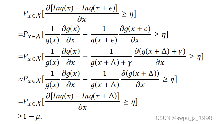
按照定理1中相同的证明程序，我们有
$$P_{x\in {\mathcal{X}}_{trap}}[\frac{\partial [\ln g(x)-\ln g(x+ϵ)]}{\partial x}\ge \eta ]\ge 1-\mu$$
因为 ${\mathcal{X}}_{trap}$ 和 ${\mathcal{X}}_{attack}$ 是 $\rho$-$covert$， 那么对于随机事件 $C\in \Omega$，$P_{x\in {\mathcal{X}}_{attack}}(C)$ 和 $P_{x\in {\mathcal{X}}_{trap}}(C)$ 最大相差不会超过 $\rho$。那么让 $C$ 代表 事件: $\frac{\partial [\ln g(x)-\ln g(x+ϵ)]}{\partial x}\ge \eta$, 对于 $x\in {\mathcal{X}}_{attack}$,
$$\begin{gathered} P_{x\in {\mathcal{X}}_{attack}}[\frac{\partial [\ln g(x)-\ln g(x+ϵ)]}{\partial x}\ge \eta ] \\ \ge P_{x\in {\mathcal{X}}_{trap}}[\frac{\partial [\ln g(x)-\ln g(x+ϵ)]}{\partial x}\ge \eta ]-\rho \\ \ge 1-(\mu +\rho ) \end{gathered}$$
  定理 2 意味着当模型所有者扩展用于注入 trapdoor 的样本数据 ${\mathcal{X}}_{trap}$ 的多样性和大小时，它允许对 $y_t$ 找到一个基于梯度或基于优化的搜索的更强大和更丰富的扰动 $ϵ$。这增加了对抗样本落入“陷阱”并因此被我们检测到的机会。

2022-05-24

尝试复现文章的工作，下面是生成 trapdoor 中的 mask 和 pattern 的核心代码

def construct_mask_random_location(image_row=32, image_col=32, channel_num=3, pattern_size=4,
                                   color=[255.0, 255.0, 255.0]):
    c_col = random.choice(range(0, image_col - pattern_size + 1))
    c_row = random.choice(range(0, image_row - pattern_size + 1))

    mask = np.zeros((image_row, image_col, channel_num))
    pattern = np.zeros((image_row, image_col, channel_num))

    mask[c_row:c_row + pattern_size, c_col:c_col + pattern_size, :] = 1
    if channel_num == 1:
        pattern[c_row:c_row + pattern_size, c_col:c_col + pattern_size, :] = [1]
    else:
        pattern[c_row:c_row + pattern_size, c_col:c_col + pattern_size, :] = color

    return mask, pattern

#target_ls 标签的个数;
#num_clusters: 如果是单标签防御，num_clusters = 1，多标签防御，num_clusters = 5(自定义) 表示有5个mask
#pattern_size: 每一个方形 mask 的像素宽度
#mask_ratio: 表示最后覆盖的比例 
#函数的返回值 total_ls 是所有标签的mask和pattern的数组
def craft_trapdoors(target_ls, image_shape, num_clusters, pattern_per_label=1, pattern_size=3, mask_ratio=0.1,
                    mnist=False):
    if mnist:
        return iter_pattern_base_per_mnist(target_ls, image_shape, num_clusters, pattern_per_label=pattern_per_label,
                                           pattern_size=pattern_size,
                                           mask_ratio=mask_ratio)
    total_ls = {}

    for y_target in target_ls:
        cur_pattern_ls = []

        for _ in range(pattern_per_label):
            tot_mask = np.zeros(image_shape)
            tot_pattern = np.zeros(image_shape)

            for p in range(num_clusters):
                mask, _ = construct_mask_random_location(image_row=image_shape[0],
                                                         image_col=image_shape[1],
                                                         channel_num=image_shape[2],
                                                         pattern_size=pattern_size)
                tot_mask += mask

                m1 = random.uniform(0, 255)
                m2 = random.uniform(0, 255)
                m3 = random.uniform(0, 255)

                s1 = random.uniform(0, 255)
                s2 = random.uniform(0, 255)
                s3 = random.uniform(0, 255)

                r = np.random.normal(m1, s1, image_shape[:-1])
                g = np.random.normal(m2, s2, image_shape[:-1])
                b = np.random.normal(m3, s3, image_shape[:-1])
                cur_pattern = np.stack([r, g, b], axis=2)
                cur_pattern = cur_pattern * (mask != 0)
                cur_pattern = np.clip(cur_pattern, 0, 255.0)
                tot_pattern += cur_pattern

                tot_mask = (tot_mask > 0) * mask_ratio
                tot_pattern = np.clip(tot_pattern, 0, 255.0)
                cur_pattern_ls.append([tot_mask, tot_pattern])

        total_ls[y_target] = cur_pattern_ls

    return total_ls

2022-05-25

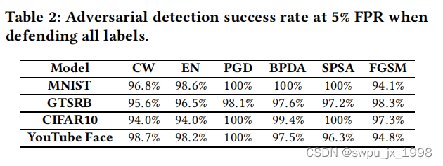
文中实验部分验证 了一下四个问题

• trapdoor模型是否能够抵御最新的攻击方式？
• trapdoor模型是否会影响正常数据的分类准确率？
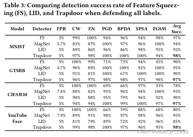
• trapdoor模型是否优于最新的对抗样本检测算法？
• 使用不同的策略生成 trapdoor signature 对模型效果有什么影响？

单标签防御对比实验

1. 在有陷阱输入和无陷阱输入的模型上，比较正常输入/陷阱输入和对抗输入/陷阱输入之间的余弦相似度。
   
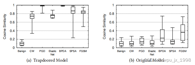
2. 检测模型在对抗输入下的准确率
   

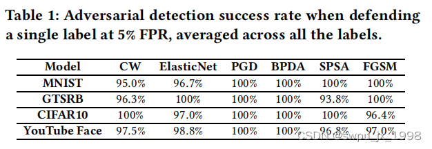
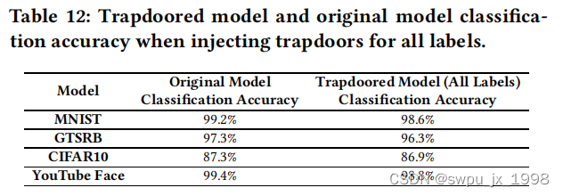
多标签防御的对比实验

1. trapdoor模型对正常数据分类效果的影响
   
2. 不同攻击对抗样本的检测准确率
   
3. 与其他三种先进的检测算法的效果对比
   
4. 不同 trapdoor signatures 的检测效果，修改策略有两种（1）用不同的神经网络层的激活特征作为$g(x)$。（2）选择不同的神经元的个数。
   
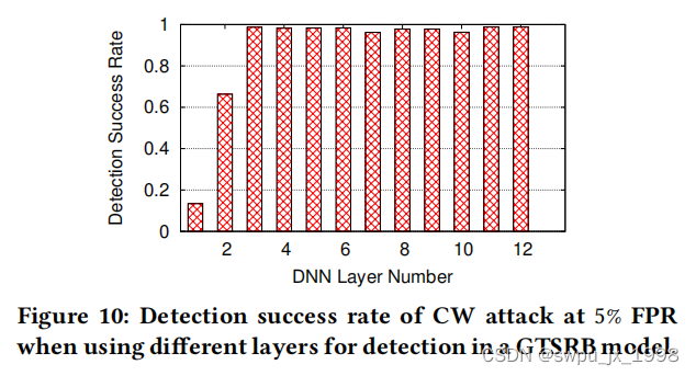
   实验结果表明使用 GTSRB 模型的不同层计算神经元特征时的检测成功率。 通过前两个卷积层，所有后面的层在 5% FPR 时导致检测成功率超过 96.20%。 更重要的是，在后面的层中选择任何随机的神经元子集会产生有效的激活特征。 具体来说，从 GTSRB 的前两层以外的任何层中采样 n 个神经元会产生一个有效的陷门签名，对抗性检测成功率始终高于 96%。

2022-05-27

def main():
    random.seed(args.seed)
    np.random.seed(args.seed)
    set_random_seed(args.seed)

    # sess = init_gpu(args.gpu)
    model = CoreModel(args.dataset, load_clean=False)
    new_model = model.model
    a = new_model.layers
    for item in a:
        print(item.output)
    target_ls = range(model.num_classes)
    INJECT_RATIO = args.inject_ratio
    print("Injection Ratio: ", INJECT_RATIO)
    f_name = "{}".format(args.dataset)

    os.makedirs(DIRECTORY, exist_ok=True)
    file_prefix = os.path.join(DIRECTORY, f_name)

    pattern_dict = craft_trapdoors(target_ls, model.img_shape, args.num_cluster,
                                   pattern_size=args.pattern_size, mask_ratio=args.mask_ratio,
                                   mnist=1 if args.dataset == 'mnist' else 0)

    RES = {}
    RES['target_ls'] = target_ls
    RES['pattern_dict'] = pattern_dict

    data_gen = ImageDataGenerator()

    X_train, Y_train, X_test, Y_test = load_dataset(args.dataset)
    train_generator = data_gen.flow(X_train, Y_train, batch_size=32)
    number_images = len(X_train)
    test_generator = data_gen.flow(X_test, Y_test, batch_size=32)

    new_model.compile(loss='categorical_crossentropy', optimizer=tf.keras.optimizers.Adam(learning_rate =lr_schedule(0)),
                      metrics=['accuracy'])

    #按照训练次数修改学习率
    lr_scheduler = LearningRateScheduler(lr_schedule)

    lr_reducer = ReduceLROnPlateau(factor=np.sqrt(0.1),
                                   cooldown=0,
                                   patience=5,
                                   min_lr=0.5e-6)

    base_gen = DataGenerator(target_ls, pattern_dict, model.num_classes)
    test_adv_gen = base_gen.generate_data(test_generator, 1)
    test_nor_gen = base_gen.generate_data(test_generator, 0)
    clean_train_gen = base_gen.generate_data(train_generator, 0)
    trap_train_gen = base_gen.generate_data(train_generator, INJECT_RATIO)

    os.makedirs(MODEL_PREFIX, exist_ok=True)
    os.makedirs(DIRECTORY, exist_ok=True)

    model_file = MODEL_PREFIX + f_name + "_model.h5"
    RES["model_file"] = model_file

    if os.path.exists(model_file):
        os.remove(model_file)

    cb = CallbackGenerator(test_nor_gen, test_adv_gen, model_file=model_file, expected_acc=model.expect_acc)
    callbacks = [lr_reducer, lr_scheduler, cb]

    print("First Step: Training Normal Model...")
    new_model.fit(clean_train_gen, validation_data=test_nor_gen, steps_per_epoch=number_images // 32,
                            epochs=model.epochs, verbose=0, callbacks=callbacks, validation_steps=100,
                            use_multiprocessing=False,
                            workers=1)

    print("Second Step: Injecting Trapdoor...")
    new_model.fit(trap_train_gen, validation_data=test_nor_gen, steps_per_epoch=number_images // 32,
                            epochs=model.epochs, verbose=1, callbacks=callbacks, validation_steps=100,
                            use_multiprocessing=True,
                            workers=1)

    if not os.path.exists(model_file):
        raise Exception("NO GOOD MODEL!!!")

    new_model = keras.models.load_model(model_file)
    loss, acc = new_model.evaluate_generator(test_nor_gen, verbose=0, steps=100)

    RES["normal_acc"] = acc
    loss, backdoor_acc = new_model.evaluate_generator(test_adv_gen, steps=200, verbose=0)
    RES["trapdoor_acc"] = backdoor_acc

    file_save_path = file_prefix + "_res.p"
    pickle.dump(RES, open(file_save_path, 'wb'))
    print("File saved to {}, use this path as protected-path for the eval script. ".format(file_save_path))