机器学习实战(8) 利用K-means聚类算法对未标注数据分组

K-均值聚类算法

随机选择k个点为质心，依据于距离函数划分类，更新质心，划分类，直到所有样本类别不再改变。
首先构建距离计算函数和随机选取质心的函数，关于距离计算函数可以采用其他方式。

def dist(veca,vecb):
    return np.sqrt(np.sum(np.square(veca-vecb)))
def randcent(data,k):
    n = data.shape[1]
    cent = np.zeros((k,n))
    for j in range(n):
        minj = np.min(data[:,j])
        rangj = float(np.max(data[:,j]-minj))
        cent[:,j] = np.squeeze(minj + rangj*np.random.rand(k,1))
    return cent

构建k-means函数，这里注意下通过np.nonzero取某个类的值，nonzero处理后是包含array的tuple

def kmeans(data,k,distmeas=dist,crcent=randcent):
    m = data.shape[0]
    cluster = np.zeros((m,2))
    #print(data.shape)
    cent = crcent(data,k)
    changed = True
    while changed:
        changed = False
        for i in range(m):
            mindis = float('inf')
            minidx = -1
            for j in range(k):
                distji = distmeas(cent[j,:],data[i,:])
                if distji<mindis:
                    mindis = distji
                    minidx = j
            if cluster[i,0] != minidx: changed=True#所有样本不再改变，退出循环
            cluster[i,:] = minidx,mindis**2
        #print(cent)
        for cen in range(k):
            pts = data[np.nonzero(cluster[:,0]==cen)[0]]
            cent[cen,:] = np.mean(pts,0)
    return cent,cluster

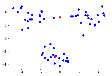
处理并画个图看下聚类情况

mycent,mycluster = kmeans(data1,2)#结果相同但顺序不同
np.sum(mycluster[:,1])
plt.figure()
plt.scatter(data1[:,0],data1[:,1],c='blue')
plt.scatter(mycent[:,0],mycent[:,1],c='red')
output:
[[ 4.0874063   2.72558262]
 [ 3.14432645 -1.73301379]]
[[ 0.12097373  3.39830046]
 [-0.60606057 -2.27031783]]
[[-0.00675605  3.22710297]
 [-0.45965615 -2.7782156 ]]

二分K-均值算法

K-均值算法容易收敛于局部最小值，这里我们介绍一种二分K-均值算法。
算法是将数据循环二分（k=2），选择使误差最小的簇进行划分操作。

#二分 K-均值算法
def bikmeans(data,k,distmeas=dist):
    m = data.shape[0]
    cluster = np.zeros((m,2))
    cent = np.mean(data,0).tolist()#初始化一个簇
    centlist = [cent]
    for i in range(m):
        cluster[i,1] = distmeas(np.array(cent),data[i,:])**2
    while (len(centlist)<k):
        lowsse = float('inf')
        for i in range(len(centlist)):
            ptscluster = data[np.nonzero(cluster[:,0]==i)[0],:]#获取一个分类的数据
            centtoid,splitclus = kmeans(ptscluster,2,distmeas)#执行分类获取质心和聚类结果（包含方差）
            ssesplit = np.sum(splitclus[:,1])
            ssenotsplit = np.sum(cluster[np.nonzero(cluster[:,0]!=i)[0],1])
            #if ssenotsplit<0: print(data[np.nonzero(cluster[:,0]!=i)[0],1])这里把cluster输成data导致ssenotsplit一直有负的...
            print('ssesplit,ssenotsplit',ssesplit,ssenotsplit)
            if (ssesplit+ssenotsplit)< lowsse:#比较方差和
                bestcent=i
                bestnewcents=centtoid
                bestclu=splitclus.copy()
                lowsse = ssesplit+ssenotsplit
        bestclu[np.nonzero(bestclu[:,0]==1)[0],0] = len(centlist)#若原来cnetlist有两个质心（0 1），则这个簇序列号为2
        bestclu[np.nonzero(bestclu[:,0]==0)[0],0] = bestcent#继承原来的簇序列号
        #print('the best cent to split is ',bestcent)
        #print('the len of bestclu is ',len(bestclu))
        print('the split result',len(bestclu[np.nonzero(bestclu[:,0]==bestcent)[0],0]))
        centlist[bestcent]=bestnewcents[0,:]
        centlist.append(bestnewcents[1,:])
        cluster[np.nonzero(cluster[:,0]==bestcent)[0],:] = bestclu#cluster[cluster[:,0]==bestcent,:] = bestclu
    return np.array(centlist),cluster

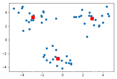
测试一下，结果图如下：

bicent,bicluster = bikmeans(data1,3)
plt.figure()
plt.scatter(data1[:,0],data1[:,1])
plt.scatter(bicent[:,0],bicent[:,1],c='red',s=90,marker='s')

接下来实例应用，对地理坐标进行聚类。
重新定义一个距离函数，通过经纬度计算距离

def distslc(veca,vecb): 
    a = np.sin(veca[1]*np.pi/180)*np.sin(vecb[1]*np.pi/180)
    b = np.cos(veca[1]*np.pi/180)*np.cos(vecb[1]*np.pi/180)*np.cos(np.pi*(vecb[0]-veca[0])/180)
    return np.arccos(a+b)*6371.0#向量外积

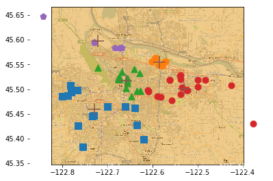
对地理坐标进行聚类

执行聚类，并将聚类结果更新在地图上。

def cluclub(filename,num=5):
    datlist = []
    with open(filename) as fr:
        for line in fr.readlines():
            linearr = line.split('\t')
            datlist.append([float(linearr[4]),float(linearr[3])])
    data = np.array(datlist)
    mycent,cluster = bikmeans(data,num,distmeas=distslc)
    fig=plt.figure()
    rect = [0.1,0.1,0.8,0.8]#l,b,w,h
    scmaker = ['s','o','^','8','p','d','v','h','>','<']
    axprops = dict(xticks=[],yticks=[])
    ax0=fig.add_axes(rect,label='ax0',**axprops)#在位置rect增加一个坐标轴
    imgp = plt.imread('/Users/enjlife/machine-learning/machinelearninginaction/ch10/Portland.png')
    ax0.imshow(imgp)#显示图片
    ax1=fig.add_axes(rect,label='ax1',frameon=False)
    for i in range(num):
        ptsclu = data[np.nonzero(cluster[:,0]==i)[0],:]#获取每一个簇，对于每一个簇画一个style
        mastyle = scmaker[i%len(scmaker)]
        ax1.scatter(ptsclu[:,0],ptsclu[:,1],marker=mastyle,s=90)
    ax1.scatter(mycent[:,0],mycent[:,1],marker='+',s=300)#画出质心
    plt.show()
cluclub(filename4,num=5)
output:
ssesplit,ssenotsplit 3043.263315808114 0.0
the split result 0.0
ssesplit,ssenotsplit 1321.0446322860967 851.4388885636852
ssesplit,ssenotsplit 501.3287881573154 2191.824427244429
the split result 0.0
ssesplit,ssenotsplit 245.684452017245 1594.360070185498
ssesplit,ssenotsplit 494.98425059436954 1321.0446322860967
ssesplit,ssenotsplit 410.1002223672573 1429.5623392279695
the split result 10.0
ssesplit,ssenotsplit 275.855667749565 1237.9054322161824
ssesplit,ssenotsplit 2.2994326371319347 1806.193631225216
ssesplit,ssenotsplit 279.34928298338923 1073.1077012586538
ssesplit,ssenotsplit 313.49641740579887 1330.879883941347
the split result 36.0

未完待续…