基于可解释性深度学习的马铃薯叶病害检测

数据集来自kaggle文章，代码较为简单。

import numpy as np # linear algebra
import pandas as pd # data processing, CSV file I/O (e.g. pd.read_csv)


# Input data files are available in the read-only "../input/" directory
# For example, running this (by clicking run or pressing Shift+Enter) will list all files under the input directory


import os
for dirname, _, filenames in os.walk('/kaggle/input'):
    for filename in filenames:
        print(os.path.join(dirname, filename))

Neural Network Model with TensorFlow and Keras for Classification

import tensorflow as tf
from tensorflow.keras import models,layers
import matplotlib.pyplot as plt


BATCH_SIZE=32
IMAGE_SIZE=224
CHANNELS=3
EPOCHS=50

Loading Image Dataset for Training

dataset=tf.keras.preprocessing.image_dataset_from_directory(
    "/kaggle/input/potato-dataset/PlantVillage",
    shuffle=True,
    image_size=(IMAGE_SIZE,IMAGE_SIZE),
    batch_size=BATCH_SIZE
)

Retrieving Class Names from the Dataset

class_names=dataset.class_names
class_names

Data Visualization

import os


Potato___Early_blight_dir = '/kaggle/input/potato-dataset/PlantVillage/Potato___Early_blight'
Potato___Late_blight_dir = '/kaggle/input/potato-dataset/PlantVillage/Potato___Late_blight'
Potato___healthy_dir = '/kaggle/input/potato-dataset/PlantVillage/Potato___healthy'
import matplotlib.pyplot as plt


# Define the categories and corresponding counts
categories = ['Early Leaf Blight','Late Leaf Blight','Healthy']
counts = [len(os.listdir(Potato___Early_blight_dir)), len(os.listdir(Potato___Late_blight_dir)), len(os.listdir(Potato___healthy_dir))]


# Create a bar plot to visualize the distribution of images
plt.figure(figsize=(12, 6))
plt.bar(categories, counts, color='skyblue')
plt.xlabel('Categories')
plt.ylabel('Number of Images')
plt.title('Distribution of Images in Different Categories')
plt.show()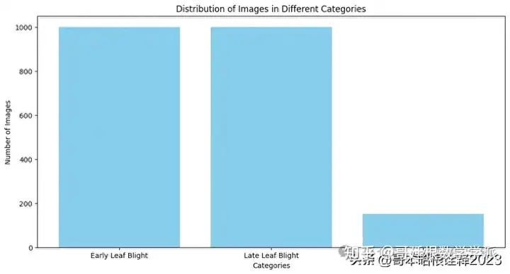

Visualizing Sample Images from the Dataset

plt.figure(figsize=(10,10))
for image_batch, labels_batch in dataset.take(1):
    print(image_batch.shape)
    print(labels_batch.numpy())
    for i in range(12):
        ax=plt.subplot(3,4,i+1)
        plt.imshow(image_batch[i].numpy().astype("uint8"))
        plt.title(class_names[labels_batch[i]])
        plt.axis("off")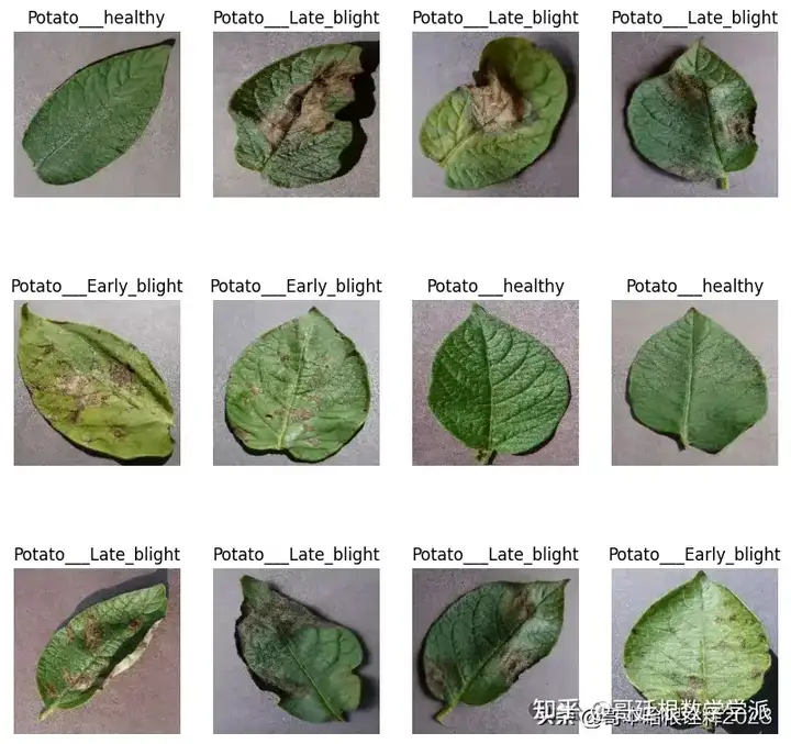

Function to Split Dataset into Training and Validation Set

def get_dataset_partitions_tf(ds, train_split=0.8, val_split=0.2, shuffle=True, shuffle_size=10000):
    assert(train_split+val_split)==1


    ds_size=len(ds)


    if shuffle:
        ds=ds.shuffle(shuffle_size, seed=12)


    train_size=int(train_split*ds_size)
    val_size=int(val_split*ds_size)


    train_ds=ds.take(train_size)
    val_ds=ds.skip(train_size).take(val_size)


    return train_ds, val_ds
train_ds, val_ds =get_dataset_partitions_tf(dataset)

Data Augmentation

train_ds= train_ds.cache().shuffle(1000).prefetch(buffer_size=tf.data.AUTOTUNE)
val_ds= val_ds.cache().shuffle(1000).prefetch(buffer_size=tf.data.AUTOTUNE)
for image_batch, labels_batch in dataset.take(1):
    print(image_batch[0].numpy()/255)
pip install preprocessing
resize_and_rescale = tf.keras.Sequential([
    layers.Resizing(IMAGE_SIZE, IMAGE_SIZE),
    layers.Rescaling(1./255),
])
data_augmentation=tf.keras.Sequential([
    layers.RandomFlip("horizontal_and_vertical"),
    layers.RandomRotation(0.2),
])
n_classes=3

Our own Convolutional Neural Network (CNN) for Image Classification

input_shape=(BATCH_SIZE, IMAGE_SIZE,IMAGE_SIZE,CHANNELS)
n_classes=3


model_1= models.Sequential([
    resize_and_rescale,
    data_augmentation,
    layers.Conv2D(32, kernel_size=(3,3), activation='relu', input_shape=input_shape),
    layers.MaxPooling2D((2,2)),
    layers.Conv2D(64, kernel_size=(3,3), activation='relu'),
    layers.MaxPooling2D((2,2)),
    layers.Conv2D(64, kernel_size=(3,3), activation='relu'),
    layers.MaxPooling2D((2,2)),
    layers.Conv2D(64, (3,3), activation='relu'),
    layers.MaxPooling2D((2,2)),
    layers.Conv2D(64, (3,3), activation='relu'),
    layers.MaxPooling2D((2,2)),
    layers.Conv2D(128, (3,3), activation='relu'),
    layers.MaxPooling2D((2,2)),
    layers.Flatten(),
    layers.Dense(256,activation='relu'),
    layers.Dense(n_classes, activation='softmax'),
])
model_1.build(input_shape=input_shape)
model_1.summary()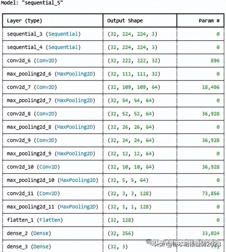

model_1.compile(
    optimizer='adam',
    loss=tf.keras.losses.SparseCategoricalCrossentropy(from_logits=False),
    metrics=['accuracy']
)
history=model_1.fit(
    train_ds,
    batch_size=BATCH_SIZE,
    validation_data=val_ds,
    verbose=1,
    epochs=50
)
scores=model_1.evaluate(val_ds)

Training History Metrics Extraction

acc=history.history['accuracy']
val_acc=history.history['val_accuracy']


loss=history.history['loss']
val_loss=history.history['val_loss']
history.history['accuracy']

Training History Visualization

EPOCHS=50
plt.figure(figsize=(20,8))
plt.subplot(