


吴恩达机器学习 Chapter7 逻辑回归 (Logistic Regression)
Classification
Classification is the main application of Logistic Regression.
Hypothesis Representation
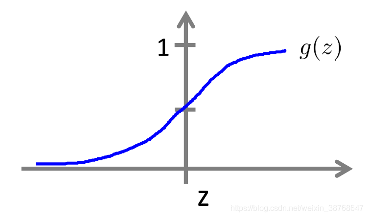
Logistic/Sigmoid function
g
(
z
)
=
1
1
+
e
−
z
g(z) = \frac{1}{1+e^{-z}}
g(z)=1+e−z1
h
θ
(
x
)
=
g
(
θ
T
X
)
h_\theta(x) = g(\theta^TX)
hθ(x)=g(θTX)
h
θ
(
x
)
=
1
1
+
e
−
θ
T
X
h_\theta(x) = \frac{1}{1+e^{-\theta^TX}}
hθ(x)=1+e−θTX1
Interpretation of hypothesis
h θ ( x ) = h_\theta(x) = hθ(x)= estimated probability that y = 1 y=1 y=1 on input x x x
Decision Boundary
Decision boundary is the property of the hypothesis, not the property of data set.
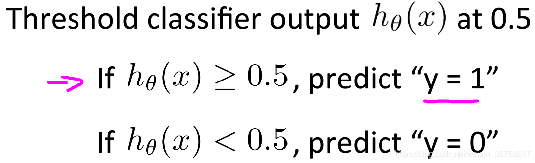
Predict:
- " y=1 " if h θ ( x ) ≥ 0.5 h_\theta(x) \geq 0.5 hθ(x)≥0.5 => θ T X ≥ 0 \theta^TX \geq 0 θTX≥0
- " y=0 " if h θ ( x ) ≤ 0.5 h_\theta(x) \leq 0.5 hθ(x)≤0.5 => θ T X ≤ 0 \theta^TX \leq 0 θTX≤0
Non-linear boundaries
E.g.
h
θ
(
x
)
=
g
(
θ
0
+
θ
1
x
1
+
θ
2
x
2
+
θ
3
x
1
2
+
θ
4
x
2
2
)
h_\theta(x) = g(\theta_0 + \theta_1x_1 + \theta_2x_2+\theta_3x_1^2+\theta_4x_2^2)
hθ(x)=g(θ0+θ1x1+θ2x2+θ3x12+θ4x22)
Decision boundaries can be more complex: higher order polynomial features.
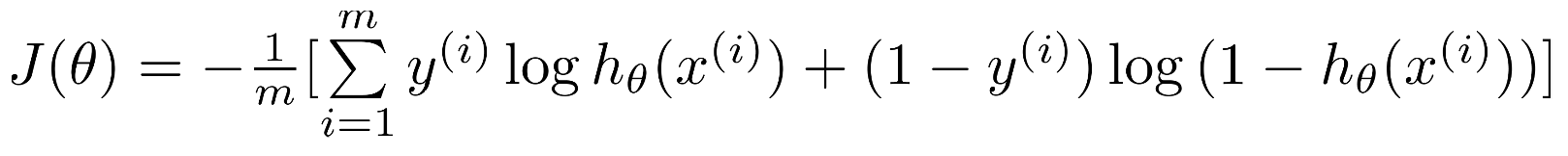
Cost function
Square error function is not convex.
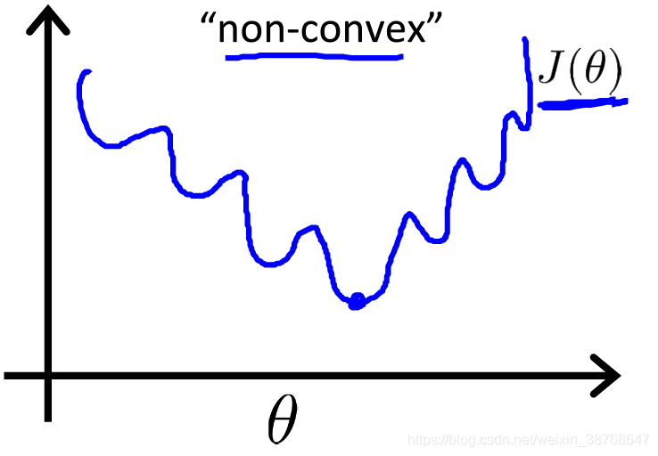
Cannot apply old version directly.
Use log
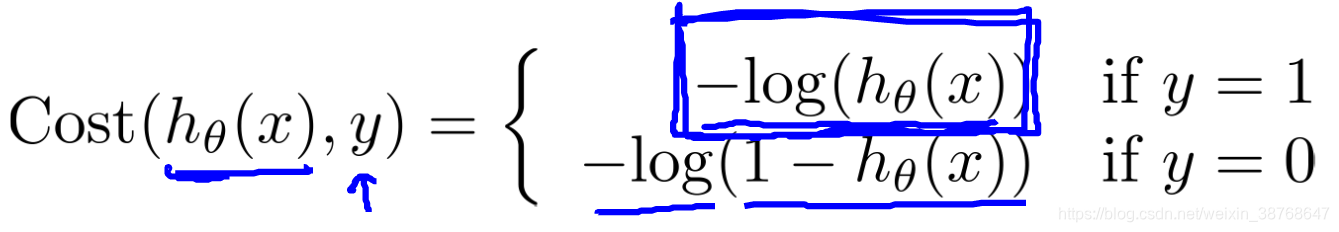
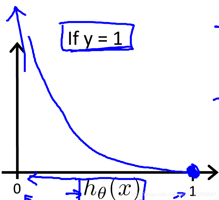
Intuition
If
h
θ
(
x
)
=
0
h_\theta(x) = 0
hθ(x)=0(predict y = 0), but actually
y
=
1
y = 1
y=1, then we’ll penalize learning algorithm by a very large cost.
Simplified cost function
C o s t ( h θ ( x ) , y ) = − y l o g h θ ( x ) − ( 1 − y ) l o g ( 1 − h θ ( x ) ) Cost(h_\theta(x), y) = -ylogh_\theta(x)-(1-y)log(1-h_\theta(x)) Cost(hθ(x),y)=−yloghθ(x)−(1−y)log(1−hθ(x))
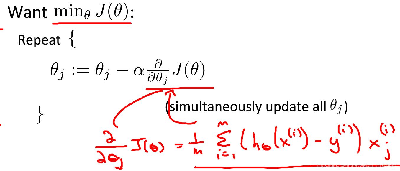
Gradient descent
Want
m
i
n
J
(
θ
)
min J(\theta)
minJ(θ):
∂
J
(
θ
)
∂
θ
i
=
1
m
∑
(
−
y
1
h
θ
(
x
)
−
1
−
y
1
−
h
θ
(
x
)
(
−
1
)
)
∂
h
θ
(
x
)
∂
θ
i
=
1
m
∑
(
−
y
1
h
θ
(
x
)
+
1
−
y
1
−
h
θ
(
x
)
)
(
−
1
(
1
+
e
−
θ
T
x
)
2
)
e
−
θ
T
x
(
−
x
)
=
1
m
∑
(
−
y
(
1
+
e
−
θ
T
x
)
+
1
−
y
1
−
1
1
+
e
−
θ
T
x
)
(
x
(
1
+
e
−
θ
T
x
)
2
)
e
−
θ
T
x
=
1
m
∑
(
−
y
(
e
−
θ
T
x
)
(
1
+
e
−
θ
T
x
)
+
1
−
y
1
+
e
−
θ
T
x
)
x
=
1
m
∑
(
−
y
(
e
−
θ
T
x
+
1
)
+
1
(
1
+
e
−
θ
T
x
)
)
x
=
1
m
∑
(
h
θ
(
x
)
−
y
)
x
\begin{aligned} \frac{\partial J(\theta)}{\partial\theta_i}&=\frac{1}{m}\sum(-y \frac{1}{h_\theta(x)}-\frac{1-y}{1-h_\theta(x)}(-1))\frac{\partial h_\theta(x)}{\partial \theta_i} \\ &= \frac{1}{m}\sum(-y \frac{1}{h_\theta(x)}+\frac{1-y}{1-h_\theta(x)})(-\frac{1}{(1+e^{-\theta^Tx})^2})e^{-\theta^Tx}(-x) \\ &=\frac{1}{m}\sum(-y (1+e^{-\theta^Tx})+\frac{1-y}{1-\frac{1}{1+e^{-\theta^Tx}}})(\frac{x}{(1+e^{-\theta^Tx})^2})e^{-\theta^Tx} \\ &= \frac{1}{m}\sum(\frac{-y(e^{-\theta^Tx})}{(1+e^{-\theta^Tx})}+\frac{1-y}{1+e^{-\theta^Tx}})x \\ &= \frac{1}{m}\sum(\frac{-y(e^{-\theta^Tx}+1)+1}{(1+e^{-\theta^Tx})})x \\ &= \frac{1}{m}\sum(h_\theta(x)-y)x\end{aligned}
∂θi∂J(θ)=m1∑(−yhθ(x)1−1−hθ(x)1−y(−1))∂θi∂hθ(x)=m1∑(−yhθ(x)1+1−hθ(x)1−y)(−(1+e−θTx)21)e−θTx(−x)=m1∑(−y(1+e−θTx)+1−1+e−θTx11−y)((1+e−θTx)2x)e−θTx=m1∑((1+e−θTx)−y(e−θTx)+1+e−θTx1−y)x=m1∑((1+e−θTx)−y(e−θTx+1)+1)x=m1∑(hθ(x)−y)x
Algorithm
Advanced optimization
- Gradient descent
- Conjugate gradient
- BFGS
- L-BFGS
Advantages:
- No need to manually pick α \alpha α => A clever innerloop that can automatically choose α \alpha α
- Often faster than gradient descent
Disadvantages
- More complex
Multi-class classification One-vs-all
Fit m classifiers that try to estimate what is the probability that P ( y = 1 ∣ x ; θ ) P(y=1|x;\theta) P(y=1∣x;θ)
One-vs-all
Train a logistic regression classifier
h
θ
i
(
x
)
h_\theta^i(x)
hθi(x) for each i to predict the probability that
y
=
i
y=i
y=i.
To predict:
On a new input x, pick the class i that maximizes
m
a
x
i
h
θ
(
i
)
(
x
)
max_ih_\theta^{(i)}(x)
maxihθ(i)(x)


 1138
1138

 被折叠的 条评论
为什么被折叠?
被折叠的 条评论
为什么被折叠?
 到【灌水乐园】发言


