####设置随机数种子 使结果可重复####
set.seed(12345)
library(Seurat)
library(tidyverse)
library(magrittr)
library(RColorBrewer)
library(reshape2)
library(Biobase)
library(ggsci)
library(ggpubr)
library(data.table)
library(monocle)
library(Matrix)
library(writexl)
读取.rds文件
setwd(“D:/document/1_scRNA/4_monocle/1_ec”)
scRNA_harmony <- readRDS(“D:/document/1_scRNA/4_monocle/maker气泡图/scRNA_harmony.rds”)
#分类
new.cluster.ids <- c(“0”= “EC”,
“1”= “MC”,
“2”= “VC”,
“3”= “MC”,
“4”= “EC”,
“5”= “PC”,
“6”= “UN”,
“7”= “MC”,
“8”= “VC”,
“9”= “PC”,
“10”= “MC”,
“11”= “PC”,
“12”= “VC”,
“13”= “TRI”,
“14”= “VC”)
将新的细胞类型标签存储到 meta.data 中
scRNA_harmony@meta.data$celltype <- new.cluster.ids[as.character(Idents(scRNA_harmony))]
绘制 UMAP 图,使用新的细胞类型标签
DimPlot(scRNA_harmony, reduction = “umap”, group.by = “celltype”, label = TRUE, label.size = 4)
#创建monocle对象
unique(scRNA_harmony$seurat_clusters)
#01选择需要构建细胞分化轨迹的细胞类型(subset提取感兴趣的名字,上面已经准备好名字了
seurat=subset(scRNA_harmony, idents = c( “0”, “4”,“13”))
unique(seurat$seurat_clusters)
table(seurat$seurat_clusters)
#0 1 2 3 4 5 6 7 8 9 10 11 12 13 14
#0 0 4696 0 0 3058 0 0 1933 1108 0 711 536 0 369
#load(“D:/document/2_scRNAseq/4_2412SCZ/scrna2.RData”)
#SCT是标准化后的数据,RNA是原始数据
#load(“D:/document/2_scRNAseq/1_SC/BMC_KW_monocle_over.RData”)
#02构建monocle独有的celldata对象
expr_matrix=seurat@assays$SCT@counts#使用counts表达值(第一个准备文件:基因count矩阵)
####转换为稀疏矩阵####
如果 expr_matrix 是稠密矩阵(dense matrix),转换为稀疏矩阵
if (!is(expr_matrix, “sparseMatrix”)) {
expr_matrix <- as(expr_matrix, “dgCMatrix”)
}
sample_sheet <- seurat@meta.data#将实验信息赋值新变量(第二个准备文件:细胞表型信息-metadata)
#gene_annotation=data.frame(gene_short_name=rownames(seurat))构建一个含有基因名字的数据框
因为默认从RNA中提取细胞信息,所以需要从 SCT assay 中提取基因名
gene_annotation <- data.frame(gene_short_name = rownames(seurat@assays$SCT))
rownames(gene_annotation) <- rownames(seurat@assays$SCT)#(第三个文件:基因名为行名的基因名数据框)
pd <- new(“AnnotatedDataFrame”,data= sample_sheet)#将实验信息变量转化为monocel可以接收的对象
fd <- new(“AnnotatedDataFrame”,data=gene_annotation)#将基因注释变量转化为monocle可以接收的对象
cds <- newCellDataSet(expr_matrix, phenoData = pd, featureData = fd,expressionFamily=negbinomial.size())#创建一个monocle的对象
#cds cellData对象,monocle独有
#03相当于归一化Size factors帮助标准化基因在细胞间的差异,"dispersion"值帮助后面的差异表达分析执行。
cds <- estimateSizeFactors(cds)
cds <- estimateDispersions(cds)
#04数据降维,特征基因的选择
#过滤低表达基因;差异分析获得top1000排序基因(可视化用来排序的基因)
##注意 – differentialGeneTest这一步有些久
cds <- detectGenes(cds,min_expr=0.1)#统计,过滤低表达基因(表达量过滤低表达基因)
expressed_genes <- row.names(subset(fData(cds),num_cells_expressed >=10))#(数量过滤低表达基因)
diff_celltype <- differentialGeneTest(cds[expressed_genes,], fullModelFormulaStr = “~celltype”,cores=4)#差异分析,cores是处理器核数,电脑带的动可用8或者更大
head(diff_celltype)
library (writexl)
write_xlsx(diff_celltype, “1_degForCellOrdering.xlsx”)
####1.RData####
save.image(“1.RData”)
load(“1.RData”)
#选这个
diff_celltype <- diff_celltype[order(diff_celltype$qval),]#将差异基因按照q值进行升序排列
ordering_genes <- row.names(diff_celltype[1:1000,])#选择top1000个显著基因用做后续排序,这里可修改
#ordering_genes <- row.names(diff_celltype[diff_celltype$qval <0.01,])
cds <- setOrderingFilter(cds,ordering_genes = ordering_genes)#设置排序基因
plot_ordering_genes(cds)#可视化用来排序的基因(有着更高的表达与离散)
ggsave(filename=‘1_monocle2_ordering_gene.pdf’)
####选择高变基因####
#此次选择monocle选择的高变基因
#选择二、使用monocle选择的高变基因
disp_table <- dispersionTable(cds)
disp.genes <- subset(disp_table, mean_expression >= 0.1 & dispersion_empirical >= 1 * dispersion_fit)$gene_id
cds <- setOrderingFilter(cds, disp.genes)
plot_ordering_genes(cds)#以上是选择monocle选择的高变基因进行轨迹构建,上述为高变基因计算方法,monocle在选择做轨迹的基因上共提供四种方法
##使用clusters差异表达基因
library(readxl)
diff.genes <- read_excel(‘D:/document/1_scRNA/scRNA_harmony.markers.xlsx’)
diff.genes <- subset(diff.genes,p_val_adj<0.01)$gene
cds <- setOrderingFilter(cds, diff.genes)
p1 <- plot_ordering_genes(cds)
p1
##使用seurat选择的高变基因
var.genes <- VariableFeatures(scRNA_harmony)
cds <- setOrderingFilter(cds, var.genes)
p2 <- plot_ordering_genes(cds)
p2
##使用monocle选择的高变基因
disp_table <- dispersionTable(cds)
disp.genes <- subset(disp_table, mean_expression >= 0.1 & dispersion_empirical >= 1 * dispersion_fit)$gene_id
cds <- setOrderingFilter(cds, disp.genes)
p3 <- plot_ordering_genes(cds)
p3
##结果对比
p1|p2|p3
library(cowplot)
combined_plot <- plot_grid(p1, p2, p3, ncol = 3)
ggsave(“2_combined_plot.pdf”, combined_plot, width = 15, height = 5)
#数据量过大,降维选择稀疏矩阵,但似乎本来就是稀疏矩阵
cds <- reduceDimension(cds, method=‘DDRTree’)#降维
cds <- orderCells(cds)#排序
##如果这里报错,先保存数据
#保存所有对象到my_workspace.RData
save.image(file = “01_orderCells_cds.RData”)
load(file = “01_orderCells_cds.RData”)
#降级 igraph 包到一个与 Monocle 兼容的版本
#原来的包无法覆盖时可手动删除D:\software\R-4.4.0\library\igraph
#install.packages(“remotes”)
#remotes::install_version(“igraph”, version = “2.0.2”)
##install.packages(“C:/Users/19086/Desktop/maker气泡图/igraph_2.0.3.tar.gz”, repos = NULL, type = “source”)
#可视化鉴定的State
p1=plot_cell_trajectory(cds, color_by=“State”)+
theme(text=element_text(size= 18)) #设置字体大小为 18
p1
ggsave(p1,filename =‘2_monocle2_state_trajectory_p1.pdf’, width =12, height = 9)
#可视化细胞类型
p2=plot_cell_trajectory(cds, color_by=“seurat_clusters”)+
theme(text= element_text(size=18)) #设置字体大小为 18
p2
ggsave(p2, filename = ‘3_monocle2_celltype_trajectory_p2.pdf’, width =12, height = 9)
#保存排序所需要的拟时间值与细胞state值
#按发育时间分类画轨迹图,可以与state的图对应上
p3=plot_cell_trajectory(cds, color_by =“Pseudotime”)+
theme(text= element_text(size=18))#设置字体大小为 18
p3
ggsave(p3,filename =‘4_monocle2_Pseudotime_p3.pdf’, width =12, height = 9)
#因为monocle包并不会自动设置分化起点,若发现有悖于生物学常识,则需要手动设置分化起点
#指定细胞分化轨迹的起始点,即设置root cell。
#自定义了一个名为GM_state的函数,函数主要计算包含特定类型细胞最多的state,并返回state练
#即特定细胞类型最多的state为指定起点
GM_state <- function(cds){
if (length(unique(pData(cds)$State)) > 1){
T0_counts <- table(pData(cds)$State, pData(cds)$seurat_clusters)[, “0”]
return(as.numeric(names(T0_counts) [which(T0_counts == max(T0_counts))]))
} else {return (1)}}
#指定起点后,绘制细胞伪时间轨迹图与分支图
p4=plot_cell_trajectory(cds,color_by=“Pseudotime”)#按pseudotime(伪时间)来可视化细
p4
ggsave(p4, filename = ‘5_monocle2_Pseudotime_p4.pdf’, width =12, height = 9)
plot_cell_trajectory(cds,color_by=“state”)+facet_wrap(“~State”,nrow=1)
#可以用ggsci配色,也可以使用scale_color_manual()自己设置颜色
library(ggsci)
p5=plot_cell_trajectory(cds, color_by = “sample”) + scale_color_npg()
p6=plot_cell_trajectory(cds, color_by = “State”) + scale_color_nejm()
colour = c(
“#E64B35”, # 红色
“#4DBBD5”, # 蓝色
“#00A087”, # 绿色
“#3C5488”, # 深蓝色
“#F39B7F”, # 橙色
“#8491B4”, # 灰色
“#91D1C2”, # 浅绿色
“#DC0000”, # 深红色
“#7E6148”, # 棕色
“#B09C85”, # 浅棕色
“#FF7F0E”, # 橙色
“#1F77B4”, # 蓝色
“#2CA02C”, # 绿色
“#D62728”, # 红色
“#9467BD”, # 紫色
“#8C564B” # 棕色
)
p7=plot_cell_trajectory(cds, color_by = “seurat_clusters”) + scale_color_manual(values = colour)
p5
p6
p7
ggsave(“5_seurat_clusters.png”, plot = p5, width = 8, height = 6, dpi = 300)
ggsave(“6_state.png”, plot = p6, width = 8, height = 6, dpi = 300)
ggsave(“7_seurat_clusters.png”, plot = p7, width = 8, height = 6, dpi = 300)
p8 <- plot_cell_trajectory(cds, x = 1, y = 2, color_by = “seurat_clusters”) +
theme(legend.position=‘none’,panel.border = element_blank()) + #去掉第一个的legend
scale_color_manual(values = colour)
p9 <- plot_complex_cell_trajectory(cds, x = 1, y = 2,
color_by = “seurat_clusters”)+
scale_color_manual(values = colour) +
theme(legend.title = element_blank())
p8
p9
ggsave(“8_State1_tree.png”, plot = p8, width = 8, height = 6, dpi = 300)
ggsave(“9_state2_tree.png”, plot = p9, width = 8, height = 6, dpi = 300)
library(ggpubr)
df <- pData(cds)
pData(cds)取出的是cds对象中cds@phenoData@data的内容
View(df)
p <- ggplot(df, aes(Pseudotime, colour = sample, fill = sample)) +
geom_density(bw = 0.5, size = 1, alpha = 0.5) +
theme_classic2()
p
ggsave(“10_density_plot_sample.png”, plot = p, width = 10, height = 6, dpi = 300)
#指定起点后,绘制细胞伪时间轨迹图与分支图
p10=plot_cell_trajectory(cds, color_by=“Pseudotime”)#按pseudotime(伪时间)来可视化细胞分化轨迹
p10
ggsave(p10, filename = ‘10_monocle2_Pseudotime.pdf’, width = 12, height = 9)
plot_cell_trajectory(cds, color_by =“State”)+
facet_wrap(~seurat_clusters,nrow=2)#facet_wrap函数可以把每个state单独highlight
ggsave(filename = ‘11_monocle2_divid_seurat_clusters.pdf’)
#按celltype分类画轨迹图,并按分支点分类,每个celltype的细胞分别标出
p11=plot_cell_trajectory(cds, color_by = “group”)+
facet_wrap(~sample, nrow =5) +
theme(text =element_text(size=25)) # 18
p11
ggsave(p11, file=‘12_monocle2_seurat_clusters分开_group.pdf’, width = 12, height = 18)
save.image(“out1.RData”)
library (writexl)
#鉴定伪时间相关的基因,即分化过程(state)相关的差异基因,“expressed_genes [1: 1000], ”中把[1:1000]删了就是所有基因
diff_test_res=differentialGeneTest(cds[expressed_genes, ], fullModelFormulaStr = “~sm.ns(Pseudotime)”,cores=2)#鉴定伪时间相关的基因,即分化过程相关
cores = num_cores 使用可用核心数
write_xlsx(diff_test_res, “01_diff_test_res.xlsx”)
注意可以将top5g改成任何自身感兴趣的基因,进行可视化
top100g=rownames(diff_test_res[order(diff_test_res$qval),])[1:100] # top 100个显著基因
plot_genes_in_pseudotime(cds[top100g,], color_by=“orig.ident”,ncol=1)+ # top 5个显著基因,可视化,pseudotime为横坐标
#orig.ident/celltype/seurat_clusters
theme(text = element_text(size= 15))#设置字体大小为 15
ggsave(filename = ‘13_monocle_top5_significant_gene.pdf’)
top100g_df <- data.frame(Gene = top100g)
write_xlsx(top100g_df, “02_monocle_deg_top100.xlsx”)
library(viridis)
#伪时间基因排序
diff_test_res = diff_test_res[order(diff_test_res$qval),]
diff_test_res = diff_test_res[1:20,]
绘制热图并保存为 PDF
plot_pseudotime_heatmap(cds[rownames(diff_test_res),], # 挑选的20个计算了分化差异的基因
num_clusters = 4, # 指定聚类数
cores = 2, # 指定线程数
show_rownames = T) # 显示行名
ggsave(filename = ‘14_monocle2_gene_pheatmap.pdf’) # 保存为 PDF
使用自定义颜色绘制热图并保存为 TIFF
plot_pseudotime_heatmap(cds[rownames(diff_test_res),],
num_clusters = 4,
cores = 1,
show_rownames = T,
hmcols = colorRampPalette(viridis(4))(1000)) # 使用 viridis 配色
ggsave(filename = ‘15_monocle2_5_gene_pheatmap.tiff’, # 保存为 TIFF
device = “tiff”, # 指定设备为 TIFF
dpi = 300, # 设置分辨率
width = 8, # 设置宽度
height = 6) # 设置高度
save.image(“out3_monocle_diff.RData”)
load(“out3_monocle_diff.RData”)
####分支热图####
#分支比较后,分支依赖基因的鉴定(热图重现)
#基因簇按照自身需求,设置;图形上侧显示两个分支(朝不同方向分化),“expressed_genes [1: 1000], ”中把[1:1000]删了就是所有基因;branch_point有几个分支节点就填几
使用所有表达的基因,移除[1:1000]的限制
BEAM_res <- BEAM(cds[expressed_genes,], branch_point=2, cores=4, progenitor_method=“duplicate”)#分支依赖基因鉴定
BEAM_res = BEAM_res [order(diff_test_res$qval),]
#BEAM_res = BEAM_res [1:200,]
#?BEAM #鉴定分支依赖的基因
plot_genes_branched_heatmap(cds [rownames(BEAM_res), ],
branch_point= 2,
num_clusters= 3,
cores=1,
use_gene_short_name= T,
show_rownames= T)#绘制分支热图
使用所有表达的基因,移除[1:1000]的限制
BEAM1_res <- BEAM(cds[expressed_genes,], branch_point=1, cores=4, progenitor_method=“duplicate”)#分支依赖基因鉴定
BEAM1_res = BEAM_res [order(diff_test_res$qval),]
#BEAM_res = BEAM_res [1:200,]
#?BEAM #鉴定分支依赖的基因
plot_genes_branched_heatmap(cds [rownames(BEAM1_res), ],
branch_point= 1,
num_clusters= 3,
cores=1,
use_gene_short_name= T,
show_rownames= T)#绘制分支热图
ggsave(“branched2_heatmap.jpg”, p20, width = 8, height = 6)
save.image(“out.RData”)
load(“D:/document/1_scRNA/4_monocle/1_ec/out.RData”)
怎么看不同state中我想关注的许多基因在不同group中的表达情况
最新发布


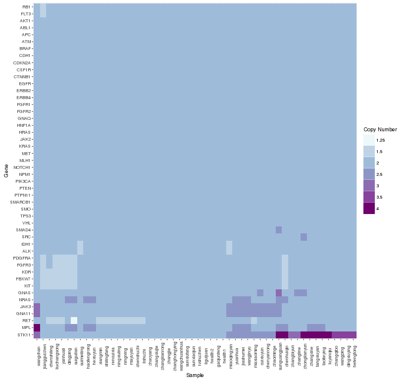
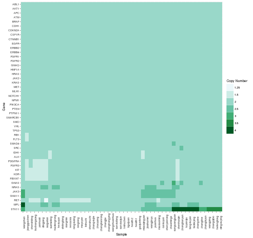
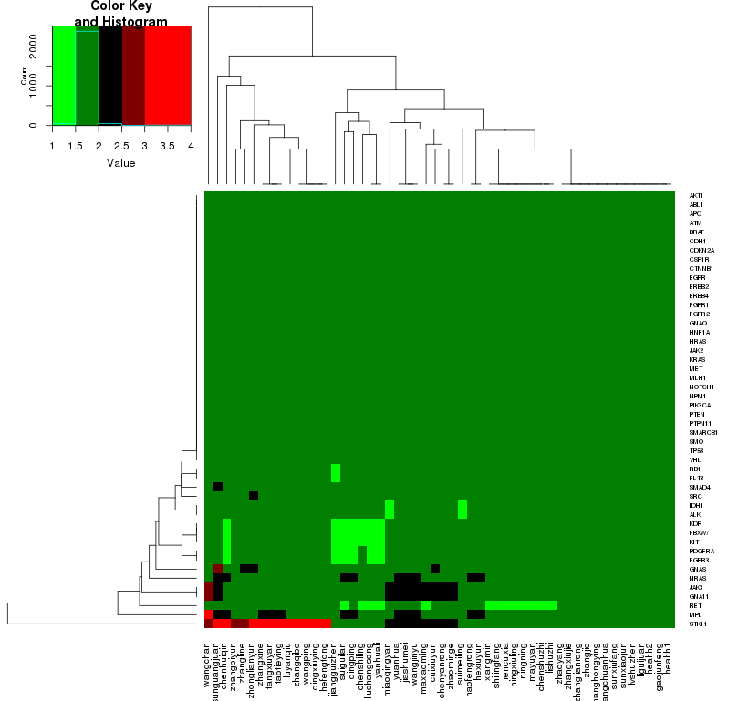
 本文详细介绍使用R语言中的pheatmap、ggplot2及gplots包绘制热图的方法。包括数据预处理、矩阵构建、不同包下的热图绘制流程及参数设置等关键步骤。


 576
576

 被折叠的 条评论
为什么被折叠?
被折叠的 条评论
为什么被折叠?
 到【灌水乐园】发言


