机器学习笔记

1. 梯度下降法

当\(n \geq 1\)时：

\(\theta_j := \theta_j - \alpha \frac{1}{m} \sum_{i=1}^m (h_\theta(x^{(i)}) - y^{(i)}) x^{(i)}_j\)

例如：

\(\theta_0 := \theta_0 - \alpha \frac{1}{m} \sum_{i=1}^m (h_\theta(x^{(i)}) - y^{(i)}) x^{(i)}_0\)

\(\theta_1 := \theta_1 - \alpha \frac{1}{m} \sum_{i=1}^m (h_\theta(x^{(i)}) - y^{(i)}) x^{(i)}_1\)

利用偏导数对参数进行迭代更新，参数\(\vec\theta\)沿着代价函数(cost function)的梯度下降，逐渐接近代价函数的极值。

---

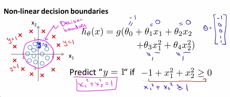
2. Logistic Regression

1. 定义：

   \(h_\theta(x)=g(\theta^Tx)\),

   \(g(z)=\cfrac1{1+e^{-z}}\)

2. 逻辑回归中：

   \(h_\theta (x) =\) (当输入为x时，\(y = 1\)的）概率

   即\(h_\theta (x) = P( y=1|x;\theta)\)

   且$ P( y=0|x;\theta)+P( y=1|x;\theta)=1$

3. decision boundary 决策边界

   

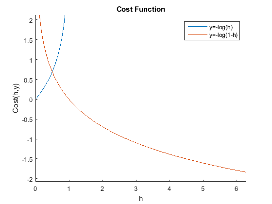
4. logistic regression cost function 逻辑回归代价函数
   \(J(\theta)=\frac1m\sum_{i=1}^mCost(h\theta(x^{(i)},y^{(i)}))\)

   \(Cost(h_\theta(x),y) = \begin{cases} -log(h_\theta(x)) & \text{if $y=1$} \\ -log(1-h_\theta(x)) & \text{if $y=0$} \\ \end{cases}\)

   Note: y = 0 or 1 always

   

5. 简化的代价函数和梯度下降法

   \(Cost(h_\theta(x),y)=-ylog(h_\theta(x))\; - \; (1-y)log(1-h_\theta(x))\)

   \(\begin{align} J(\theta) = & \frac1m\sum_{i=1}^mCost(h_\theta(x),y) \\ = & -\frac1m\left[\sum_{i=1}^my^{(i)}log(h_\theta(x^{(i)}))\; - \; (1-y^{(i)})log(1-h_\theta(x^{(i)}))\right] \end{align}\)

   求得 \(\min_\theta J(\theta)\)

   通过新的x预测：

   输出\(h_\theta(x)=\cfrac1{1+e^{-\theta^Tx}}\)
   (线性假设函数：\(h_\theta(x)=\theta^Tx\))
   梯度下降法：

   Repeat {

   \(\theta_j:=\theta_j-\alpha\sum_{i=1}^m(h_\theta(x^{(i)})-y^{(i)})x^{(i)}_j\)

   所有\(\theta_j\)必须同步更新

   }

6. 高级优化算法

   Given \(\theta\), we have code that can compute

   - \(J(\theta)\)

   - \(\frac\partial{\partial\theta_j}J(\theta)\) (for j = 0,1,...,n)

   优化算法：

   - Gradient descent

   - Conjugate gradient

   - BFGS

   - L-BFGS

   后三种算法的优点：

   - 不需要选取学习率\(\alpha\)

   - 往往比梯度下降法快

   缺点：

   - 更复杂

转载于:https://www.cnblogs.com/catmelo/p/5088053.html