Regularization

最新推荐文章于 2025-08-05 13:20:27 发布

转载最新推荐文章于 2025-08-05 13:20:27 发布 · 139 阅读

0 ·

CC 4.0 BY-SA版权

原文链接：http://www.cnblogs.com/casperwin/p/6408269.html

文章标签：

#人工智能 #开发工具

本文探讨了机器学习中常见的过拟合问题，并介绍了如何使用正则化技术来解决这一问题。通过调整模型复杂度并引入惩罚项，可以有效避免过拟合，提高模型泛化能力。

摘要生成于 C知道，由 DeepSeek-R1 满血版支持，前往体验 >

Overview

In Machine learning and statistics, a common task is to fit a model to a set of training data. This model can be used later to make predictions or classify new data points.

When the model fits the training data but does not have a good predicting performance and generalization power, we have an overfitting problem.

Overfitting

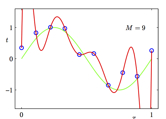
[source: Pattern Recognition and Machine Learning, Bishop, P25]

Here we are trying to do a regression on the data points (blue dots). A sine curve (green) is a reasonable fit. But we can fit it to a polynomial, and if we raise the degree of polynomial to arbitrarily high, we can reduce the error close to 0 (by Taylor expansion theorem). As shown here, the red curve is a 9-degree polynomial. Even though its root mean square error is smaller, its complexity makes it a likely result of overfitting.

Overfitting, however, is not a problem only associated with regression. It is relevant to various machine learning methods, such as maximum likelihood estimation, neural networks, etc.

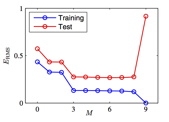
In general, it is the phenomenon where the error decreases in the training set but increases in the test set. It is captured by the plot below, which is similar to the plots in other answers.

Regulariztion

Regularization is a technique used to avoid this overfitting problem. The idea behind regularization is that models that overfit the data are complex models that have for example too many parameters.

In order to find the best model, the common method in machine learning is to define a loss or cost function that describes how well the model fits the data. The goal is to find the model that minimzes this loss function.

Regulariztion reduces overfitting by adding a complexity penalty to the loss function.

Learning performance = prediction accuracy measured on test set

Trading off complexity and degree of fit is hard.

Regularization penalizes hypothesis complexity

L2 regularization leads to small weights
L1 regularization leads to many zero weights (sparsity)

Feature selection tries to discard irrelevant features

L2 regularization: complexity = sum of squares of weights

L1 regularization (LASSO)

Dropout

Dropout is a recent technique to address the overfitting issue. It does so by “dropping out” some unit activations in a given layer, that is setting them to zero. Thus it prevents co-adaptation of units and can also be seen as a method of ensembling many networks sharing the same weights. For each training example a different set of units to drop is randomly chosen.

Dropout is a technique where randomly selected neurons are ignored during training. They are “dropped-out” randomly. This means that their contribution to the activation of downstream neurons is temporally removed on the forward pass and any weight updates are not applied to the neuron on the backward pass.

Assuming we are training a neural network as below,

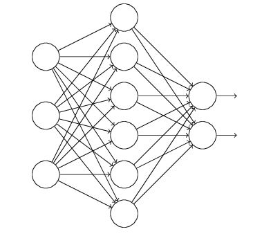
The normal process is that the raw inputs are going through the network via forward propagation and then back propagation to update the parameters and thus to learn the model. While this process is shifted as below for example after using dropout,

Firstly we remove the nodes in the hidden layer by half (here we say probability is 0.5 which is often used) and keep the input and output lays the same.
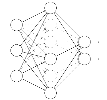
Then we make the inputs forward pass the modified neural network and back propagate through the modified neural network with obtained loss function.
Repeat the above procedures.

Using Dropout in Keras

Dropout is easily implemented by randomly selecting nodes to be dropped-out with a given probability (e.g. 20%) each weight update cycle. This is how Dropout is implemented in Keras. Dropout is only used during the training of a model and is not used when evaluating the skill of the model.

DropConnect

DropConnect by Li Wan et al., takes the idea a step further. Instead of zeroing unit activations, it zeroes the weights, as pictured nicely in Figure 1 from the paper: