Caffe solver.prototxt 文件参数解析

最新推荐文章于 2023-08-29 11:23:23 发布

原创最新推荐文章于 2023-08-29 11:23:23 发布 · 362 阅读

0 ·

CC 4.0 BY-SA版权

文章标签：

#caffe

Caffe 专栏收录该内容

1 篇文章

订阅专栏

本文详细介绍了Caffe中Solver的重要作用，它是训练神经网络过程中的核心，负责协调网络的前向传播和反向传播，通过优化算法更新参数以最小化损失。Solver配置文件solver.prototxt定义了训练参数，如学习率、优化策略和迭代次数等。文中还举例说明了各参数的具体含义和计算方法，包括学习率衰减策略、测试间隔和动量等，并提供了MNIST实例进行解析。

solver 算是 Caffe 的核心的核心，它协调着整个模型的运作。Caffe 程序运行必带的一个参数就是solver 配置文件，solver.prototxt 文件是用来告诉 Caffe 如何训练网络的。

在Deep Learning中，往往loss function是非凸的，没有解析解，我们需要通过优化方法求解。solver的主要作用就是交替调用前向（forword）算法和后向（backward）算法来更新参数，从而最小化loss，实际上就是一种迭代的优化算法。

2. solver文件介绍

Solver的流程：

设计好需要优化的对象，以及用于学习的训练网络和用于评估的测试网络。（通过调用另外一个配置文件prototxt来进行）
通过forward和backward迭代的进行优化来跟新参数。
定期的评价测试网络。（可设定多少次训练后，进行一次测试）
在优化过程中显示模型和solver的状态

在每一次的迭代过程中，solver做了这几步工作：

1、调用forward算法来计算最终的输出值，以及对应的loss

2、调用backward算法来计算每层的梯度

3、根据选用的slover方法，利用梯度进行参数更新

4、记录并保存每次迭代的学习率、快照，以及对应的状态。

solver.prototxt是caffe的配置文件。里面定义了网络训练时候的各种参数，比如学习率、权重衰减、迭代次数等等。

solver文件示例

solver文件是训练网络所必须要的文件，其中定义了诸如：求解器类型、学习率、学习率的变化策略等。其命令行调用方式模式一般为：

caffe train --solver=*_slover.prototxt

接下来看一个solver配置文件的例子：

train_net: "train.prototxt"
test_net: "val.prototxt"
test_iter: 100
test_interval: 938
base_lr: 0.00999999977648
display: 1000
max_iter: 9380
lr_policy: "step"
gamma: 0.10000000149
momentum: 0.899999976158
weight_decay: 0.000500000023749
stepsize: 3000
snapshot: 4000
snapshot_prefix: "./snapshot/"
solver_mode: GPU
type: "SGD"

下面的内容将会详细讲解其中的参数，并介绍其其使用方法。

3. solver文件参数详细解析

solver文件示例

下面以 Caffe 中的 mnist 实例进行简单明了的解释：

net: "examples/mnist/lenet_train_test.prototxt"
test_iter: 100
test_interval: 500
base_lr: 0.01
momentum: 0.9
weight_decay: 0.0005
lr_policy: "inv"
gamma: 0.0001
power: 0.75
display: 100
max_iter: 10000
snapshot: 5000
snapshot_prefix: "examples/mnist/lenet" 
solver_mode: GPU

第1行：

net: "examples/mnist/lenet_train_test.prototxt"

用于设置深度网络模型，即指定网络配置文件（该实例中为 lenet_train_test.prototxt）的路径。

第2行，第3行以及第11行：

2.    test_iter: 100
3.     test_interval: 500
11.  max_iter: 10000

test_iter 的大小为 test 数据集的总样本数与 batch_size 的比值，比如在 mnist 数据集中，有10000个测试样本，batch_size设为100的话，则 test_iter = 10000/100 = 100；

test_interval 表示测试间隔，例如，想要完成一次完整的 train 再测试，则 test_interval 的值为 50000/100 = 500，其中，50000为训练集数量，100为 batch_size 的大小；

max_iter 表示最大训练迭代次数，若 test_interval 测试间隔设为一次完整的 train，则 max_iter = test_interval * epoch，其中，epoch为训练的轮次。

第4-9行

 1. base_lr: 0.01
 2. momentum: 0.9
 3. weight_decay: 0.0005
 4. lr_policy: "inv"
 5. gamma: 0.0001
 6. power: 0.75

base_lr 用来表示网络的初始学习率；
momentum 表示动量大小，在新的计算中要保留的前面的权重数量，通常设置为0.9；

weight_decay 表示对较大权重的惩罚（正则化）因子，防止过拟合的一个参数；

lr_policy 表示训练过程中学习率的变化方式，有如下几种：

fixed：保持 base_lr 不变.
step：如果设置为 step,则还需要设置一个 stepsize, 返回 base_lr *
gamma ^ (floor(iter / stepsize)),其中 iter 表示当前的迭代次数
exp：返回 base_lr * gamma ^ iter，iter 为当前迭代次数
inv：如果设置为 inv，还需要设置一个 power, 返回 base_lr * (1 + gamma * iter) ^ (- power)
multistep：如果设置为 multistep，则还需要设置一个 stepvalue。这个参数和 step 很相似，step 是均匀等间隔变化，而 multistep 则是根据 stepvalue 值变化
poly：学习率进行多项式误差, 返回 base_lr (1 - iter/max_iter) ^ (power)
sigmoid：学习率进行sigmod衰减，返回 base_lr ( 1/(1 + exp(-gamma * (iter - stepsize))))
以为此处设置为 “inv”，所以需要设置 gamma 和 power 值。

以为此处设置为 “inv”，所以需要设置 gamma 和 power 值。

第10行

10. display: 100

表示每训练100次，在屏幕上显示一次。如果设置为0，则不显示。

第12，13行
12. snapshot: 5000
13. snapshot_prefix: “examples/mnist/lenet”

将训练出来的 model 和 solver 状态进行保存，snapshot 用于设置训练多少次后进行保存，默认为0，不保存。snapshot_prefix 为设置保存路径。也可以设置 snapshot_format，保存的类型。有两种选择：HDF5 和 BINARYPROTO ，默认为 BINARYPROTO。

第14行

14. solver_mode: GPU

设置运行模式。默认为GPU，如果没有GPU，则需要改成CPU，否则会出错。

4. 参数补充说明

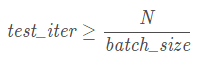
1.test_iter计算

test_iter: 100

该参数需要训练的总文件个数N和训练网络模型文件中定义的batch_size相结合，在test_iter指定的迭代次数中需要跑完所有的训练数据，这里称之为一个epoch。那么其取值可以表述为下面的公式：
在这里插入图片描述
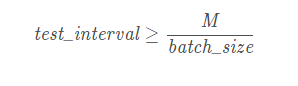
2.test_interval计算

参数test_interval，既是测试间隔，就是规定迭代多少次之后才开始进行测试

test_interval: 938

该参数的值也是与测试的总文件个数M和测试网络模型文件中定义的batch_size相结合确定的。其取值公式为：
在这里插入图片描述
3.学习率的设置及其变化策略

base_lr: 0.00999999977648 # 基础学习率
lr_policy: "step" # 学习率变化的策略
gamma: 0.10000000149 # 学习速率衰减常数，每次更新学习速率都是乘上这个固定常数
momentum: 0.899999976158 # 动量，遗忘因子
weight_decay: 0.000500000023749 # 用于防止过拟合，乘以权值惩罚项
stepsize: 3000 # 学习率变化的步长，不能太小，如果太小会导致学习率再后来越来越小，达不到充分收敛的效果。

4.求解器的类型选择

求解器的类型选择，默认就是SGD

type: "SGD"

可供选择的求解器类型：

enum SolverType {
    SGD = 0;
    NESTEROV = 1;
    ADAGRAD = 2;
    RMSPROP = 3;
    ADADELTA = 4;
    ADAM = 5;
  }

5. SolverParameter定义

这里提出完整的SolverParameter的定义，以供查阅…

// Update the next available ID when you add a new SolverParameter field.
//
// SolverParameter next available ID: 42 (last added: layer_wise_reduce)
message SolverParameter {
  //
  // Specifying the train and test networks
  //
  // Exactly one train net must be specified using one of the following fields:
  //     train_net_param, train_net, net_param, net
  // One or more test nets may be specified using any of the following fields:
  //     test_net_param, test_net, net_param, net
  // If more than one test net field is specified (e.g., both net and
  // test_net are specified), they will be evaluated in the field order given
  // above: (1) test_net_param, (2) test_net, (3) net_param/net.
  // A test_iter must be specified for each test_net.
  // A test_level and/or a test_stage may also be specified for each test_net.
  //

  // Proto filename for the train net, possibly combined with one or more
  // test nets.
  optional string net = 24;
  // Inline train net param, possibly combined with one or more test nets.
  optional NetParameter net_param = 25;

  optional string train_net = 1; // Proto filename for the train net.
  repeated string test_net = 2; // Proto filenames for the test nets.
  optional NetParameter train_net_param = 21; // Inline train net params.
  repeated NetParameter test_net_param = 22; // Inline test net params.

  // The states for the train/test nets. Must be unspecified or
  // specified once per net.
  //
  // By default, train_state will have phase = TRAIN,
  // and all test_state's will have phase = TEST.
  // Other defaults are set according to the NetState defaults.
  optional NetState train_state = 26;
  repeated NetState test_state = 27;

  // The number of iterations for each test net.
  repeated int32 test_iter = 3;

  // The number of iterations between two testing phases.
  optional int32 test_interval = 4 [default = 0];
  optional bool test_compute_loss = 19 [default = false];
  // If true, run an initial test pass before the first iteration,
  // ensuring memory availability and printing the starting value of the loss.
  optional bool test_initialization = 32 [default = true];
  optional float base_lr = 5; // The base learning rate
  // the number of iterations between displaying info. If display = 0, no info
  // will be displayed.
  optional int32 display = 6;
  // Display the loss averaged over the last average_loss iterations
  optional int32 average_loss = 33 [default = 1];
  optional int32 max_iter = 7; // the maximum number of iterations
  // accumulate gradients over `iter_size` x `batch_size` instances
  optional int32 iter_size = 36 [default = 1];

  // The learning rate decay policy. The currently implemented learning rate
  // policies are as follows:
  //    - fixed: always return base_lr.
  //    - step: return base_lr * gamma ^ (floor(iter / step))
  //    - exp: return base_lr * gamma ^ iter
  //    - inv: return base_lr * (1 + gamma * iter) ^ (- power)
  //    - multistep: similar to step but it allows non uniform steps defined by
  //      stepvalue
  //    - poly: the effective learning rate follows a polynomial decay, to be
  //      zero by the max_iter. return base_lr (1 - iter/max_iter) ^ (power)
  //    - sigmoid: the effective learning rate follows a sigmod decay
  //      return base_lr ( 1/(1 + exp(-gamma * (iter - stepsize))))
  //
  // where base_lr, max_iter, gamma, step, stepvalue and power are defined
  // in the solver parameter protocol buffer, and iter is the current iteration.
  optional string lr_policy = 8;
  optional float gamma = 9; // The parameter to compute the learning rate.
  optional float power = 10; // The parameter to compute the learning rate.
  optional float momentum = 11; // The momentum value.
  optional float weight_decay = 12; // The weight decay.
  // regularization types supported: L1 and L2
  // controlled by weight_decay
  optional string regularization_type = 29 [default = "L2"];
  // the stepsize for learning rate policy "step"
  optional int32 stepsize = 13;
  // the stepsize for learning rate policy "multistep"
  repeated int32 stepvalue = 34;

  // Set clip_gradients to &gt;= 0 to clip parameter gradients to that L2 norm,
  // whenever their actual L2 norm is larger.
  optional float clip_gradients = 35 [default = -1];

  optional int32 snapshot = 14 [default = 0]; // The snapshot interval
  optional string snapshot_prefix = 15; // The prefix for the snapshot.
  // whether to snapshot diff in the results or not. Snapshotting diff will help
  // debugging but the final protocol buffer size will be much larger.
  optional bool snapshot_diff = 16 [default = false];
  enum SnapshotFormat {
    HDF5 = 0;
    BINARYPROTO = 1;
  }
  optional SnapshotFormat snapshot_format = 37 [default = BINARYPROTO];
  // the mode solver will use: 0 for CPU and 1 for GPU. Use GPU in default.
  enum SolverMode {
    CPU = 0;
    GPU = 1;
  }
  optional SolverMode solver_mode = 17 [default = GPU];
  // the device_id will that be used in GPU mode. Use device_id = 0 in default.
  optional int32 device_id = 18 [default = 0];
  // If non-negative, the seed with which the Solver will initialize the Caffe
  // random number generator -- useful for reproducible results. Otherwise,
  // (and by default) initialize using a seed derived from the system clock.
  optional int64 random_seed = 20 [default = -1];

  // type of the solver
  optional string type = 40 [default = "SGD"];

  // numerical stability for RMSProp, AdaGrad and AdaDelta and Adam
  optional float delta = 31 [default = 1e-8];
  // parameters for the Adam solver
  optional float momentum2 = 39 [default = 0.999];

  // RMSProp decay value
  // MeanSquare(t) = rms_decay*MeanSquare(t-1) + (1-rms_decay)*SquareGradient(t)
  optional float rms_decay = 38 [default = 0.99];

  // If true, print information about the state of the net that may help with
  // debugging learning problems.
  optional bool debug_info = 23 [default = false];

  // If false, don't save a snapshot after training finishes.
  optional bool snapshot_after_train = 28 [default = true];

  // DEPRECATED: old solver enum types, use string instead
  enum SolverType {
    SGD = 0;
    NESTEROV = 1;
    ADAGRAD = 2;
    RMSPROP = 3;
    ADADELTA = 4;
    ADAM = 5;
  }
  // DEPRECATED: use type instead of solver_type
  optional SolverType solver_type = 30 [default = SGD];

  // Overlap compute and communication for data parallel training
  optional bool layer_wise_reduce = 41 [default = true];
}

<div class="hljs-button {2}" data-title="复制" data-report-click="{&quot;spm&quot;:&quot;1001.2101.3001.4259&quot;}"></div>`