斯坦福ML课程——python转写(Week4—课程作业ex3_2)_in this exercise, you will use a neural network to-优快云博客

本文链接：https://blog.youkuaiyun.com/wangzhihao_2015/article/details/103228080

本文详细介绍了利用预训练的神经网络参数进行手写数字识别的过程。通过实施前向传播算法，实现了对训练集的手写数字预测，提高了模型的准确性。文章对比了神经网络与逻辑回归在复杂假设形成上的差异，强调了神经网络处理非线性问题的能力。

摘要生成于 C知道，由 DeepSeek-R1 满血版支持，前往体验 >

利用python完成课程作业ex3的第二部分，第二部分的要求如下：

In the previous part of this exercise, you implemented multi-class logistic regression to recognize handwritten digits. However, logistic regression cannotform more complex hypotheses as it is only a linear classier.3 In this part of the exercise, you will implement a neural network to recognize handwritten digits using the same training set as before. The neural network will be able to represent complex models that form non-linear hypotheses. For this week, you will be using parameters from a neural network
that we have already trained. Your goal is to implement the feedforward propagation algorithm to use our weights for prediction. In next week's exercise, you will write the backpropagation algorithm for learning the neural network parameters.

代码如下：

# -*- coding: utf-8 -*-
"""
Created on Sat Nov 23 10:55:24 2019

@author: Lonely_hanhan
"""
import scipy.io as sio
import numpy as np
import matplotlib.pyplot as plt
import scipy.optimize as op

''' Setup the parameters you will use for this exercise '''
input_layer_size  = 400;  # 20x20 Input Images of Digits
hidden_layer_size = 25;   # 25 hidden units
num_labels = 10;          # 10 labels, from 1 to 10   
                          # (note that we have mapped "0" to label 10)

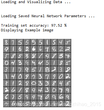
'''=========== Part 1: Loading and Visualizing Data ============='''
print('Loading and Visualizing Data ...\n')

data = sio.loadmat('D:\exercise\machine-learning-ex3\machine-learning-ex3\ex3\ex3data1.mat')
X = data['X']
y = data['y']
m = X.shape[0]

#Randomly select 100 data points to display

def displayData(X):
    
    #Compute rows, cols
    [m, n] = X.shape
    example_width = round(np.sqrt(n)).astype(int)
    example_height = (n / example_width).astype(int)
    #Compute number of items to display
    display_rows = np.floor(np.sqrt(m)).astype(int)
    display_cols = np.ceil(m / display_rows).astype(int)
    
    #Between images padding
    pad = 1
    
    #Setup blank display
    display_array = - np.ones((display_rows * (example_height + pad), \
                            display_cols * (example_width + pad)))
    
    # Copy each example into a patch on the display array
    curr_ex = 0
    for j in range(display_rows):
        for i in range(display_cols):
            if curr_ex > m-1:
                break
            #Copy the patch
            #Get the max value of the patch
            max_val = np.max(np.abs(X[curr_ex]))
            display_array[j * (example_height + pad) + np.arange(example_height),\
                          i * (example_width + pad) + np.arange(example_width)[:, np.newaxis]] = \
                          X[curr_ex].reshape((example_height, example_width)) / max_val
            curr_ex += 1
        if curr_ex > m-1:
            break
    plt.figure()
    plt.imshow(display_array, cmap='gray', extent=[-1, 1, -1, 1])
    plt.axis('off')
    return
    
    


rand_indices = np.random.permutation(range(m)) #获取0-4999 5000个无序随机索引
selected = X[rand_indices[0:100], :]  #获取前100个随机索引对应的整条数据的输入特征

displayData(selected)   #调用可视化函数 进行可视化
 
#input('Program paused. Press ENTER to continue')


# In this part of the exercise, we load some pre-initialized 
# neural network parameters.
print('\nLoading Saved Neural Network Parameters ...\n')

weight = sio.loadmat('D:\exercise\machine-learning-ex3\machine-learning-ex3\ex3\ex3weights.mat')
Theta1 = weight['Theta1'] # first layer sigmoid
Theta2 = weight['Theta2'] # second layer sigmnid

'''================= Part 3: Implement Predict ================='''

# After training the neural network, we would like to use it to predict
# the labels. You will now implement the "predict" function to use the
#  neural network to predict the labels of the training set. This lets
#  you compute the training set accuracy.
def sigmond(z):
    return 1/(1+np.exp(-z))

def predict(Theta1, Theta2, X):
    # Useful values
    m = X.shape[0]
    #num_labels = Theta2.shape[0]
    X = np.c_[np.ones(m), X]
    
    # You need to return the following variables correctly
    p = np.zeros((m, 1))
# ====================== YOUR CODE HERE ======================
# Instructions: Complete the following code to make predictions using
#               your learned neural network. You should set p to a 
#               vector containing labels between 1 to num_labels.
#
# Hint: The max function might come in useful. In particular, the max
#       function can also return the index of the max element, for more
#       information see 'help max'. If your examples are in rows, then, you
#       can use max(A, [], 2) to obtain the max for each row.
    #计算第二层
    z2 = np.dot(X, (Theta1.T))
    a2 = sigmond(z2)
    n2 = a2.shape[0]
    a2 = np.c_[np.ones(n2), a2] #第二层列加一
    #计算输出层
    z3 = np.dot(a2, Theta2.T)
    out = sigmond(z3)
    p = np.argmax(out, axis=1)
    
    return p+1

pred = predict(Theta1, Theta2, X)
print('Training set accuracy:',sum(pred[:, np.newaxis] == y)[0] /5000 * 100,"%")     

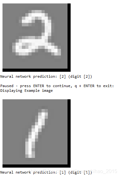
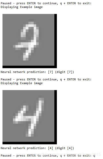
#  To give you an idea of the network's output, you can also run
# through the examples one at the a time to see what it is predicting.

# Randomly permute examples

rp = np.random.permutation(range(m))    

for i in range(m):
    print('Displaying Example image')
    example = X[rp[i]]
    example = example.reshape((1, example.size))
    displayData(example)
    plt.show()
    pred = predict(Theta1, Theta2, example)
    print('Neural network prediction: {} (digit {})'.format(pred, np.mod(pred, 10)))
 
    s = input('Paused - press ENTER to continue, q + ENTER to exit: ')
    if s == 'q':
        break

结果如下：