蒙特卡洛模拟在实际的项目管理中的应用——Python

蒙特卡洛模拟在实际的项目管理中的应用——Python

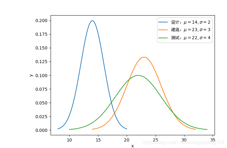
假如现在有三个项目，分别是设计、建造和测试，假设它们都是正太分布，各自的平均工期、标准差以及最悲观、最可能和最乐观的估计工期如下图所示

	最乐观	最可能	最悲观	平均工期	标准差	分布
设计	8	14	20	14	2	正太分布
建造	14	23	32	23	3	正太分布
测试	10	22	34	22	4	正太分布

我们可以先画出三个要素工期的分布

import numpy as np
import pandas as pd
import matplotlib.pyplot as plt
from scipy import stats

np.random.seed(1)
#先画出三个要素工期的正态分布概率密度图
def normplot(mu,sigma,n,name,ax):
    x = np.linspace(mu-3*sigma,mu+3*sigma,n)
    y = stats.norm.pdf(x,mu,sigma)
    #绘图需要用到latex
    ax.plot(x, y,label=r'{}：$\mu={},\sigma={}$'.format(name,mu,sigma))

fig,ax = plt.subplots(1,2,figsize=(15,5))
normplot(14, 2, 10000,'设计',ax[0])
normplot(23, 3, 10000,'建造',ax[0])
normplot(22, 4, 10000,'测试',ax[0])
ax[0].legend(prop={'family':'SimHei','size':10})
ax[0].set_xlabel('x')
ax[0].set_ylabel('y')

数学公式是用latex生成的，它是一种基于ΤΕΧ的排版系统，可以生成复杂表格和数学公式，在国外，大多高水平的论文都使用Latex对论文进行排版。Latex以其页面的美观整洁,以及功能的强大受到国际专家学者的重视。

图像如下

接下来我们就需要进行蒙特卡洛模拟，
第一步，对三个正态分布的要素的工期模拟10000次，次数越多，模拟的效果越好，得到三个要素的10000次模拟的随机工期值，
第二步，再将它们相加，就能得到总工期值，
第三步，将10000个的总工期画出它的频率直方图，注意频率直方图是指将频数除以总的观测数，就得到了每一个间隔中的频率，然后将频率除以组距（每一个间隔的宽度），所以纵坐标并不是某个值的频率，之所以要除以组距的目的是为了让频率直方图逼近于概率密度曲线，如果如果想要纵坐标为
某个区间值出现的频率，则需要将density=True，改成weights = np.ones_like(your_array)/float(len(your_array))

x1 = pd.Series(np.random.normal(loc=14,scale=2,size=10000))
x2 = pd.Series(np.random.normal(loc=23,scale=3,size=10000))
x3 = pd.Series(np.random.normal(loc=22,scale=4,size=10000))
x = x1+x2+x3
#hist()可以返回直方图的数据
n,bins,paches = ax[1].hist(x,bins=50,range=(40,80),density=True)

图形如下

根据图形可以看出，该f分布就是很明显的正太分布，但是我们想知道拟合的好不好，我们都知道根据独立正态分布可加性，可以直接计算得出总工期的均值为59，方差为29，接着我们去拟合频率直方图

mean,std = x.mean(),x.std()
y = stats.norm.pdf(bins,mean,std)
ax[1].plot(bins,y,label = r'总工期：$\mu={:.2f},\sigma={:.2f},\sigma^2={:.2f}$'.format(mean, std,std**2))
ax[1].legend(prop={'family':'SimHei','size':10})
ax[1].set_ylim(0,0.09)

图形如下

得出结论
可以模拟出来的均值和方差，与真实值还是特别接近的

完整代码如下

import numpy as np
import pandas as pd
import matplotlib.pyplot as plt
from scipy import stats

np.random.seed(1)
#先画出三个要素工期的正态分布概率密度图
def normplot(mu,sigma,n,name,ax):
    x = np.linspace(mu-3*sigma,mu+3*sigma,n)
    y = stats.norm.pdf(x,mu,sigma)
    #绘图需要用到latex
    ax.plot(x, y,label=r'{}：$\mu={},\sigma={}$'.format(name,mu,sigma))

fig,ax = plt.subplots(1,2,figsize=(15,5))
normplot(14, 2, 10000,'设计',ax[0])
normplot(23, 3, 10000,'建造',ax[0])
normplot(22, 4, 10000,'测试',ax[0])
ax[0].legend(prop={'family':'SimHei','size':10})
ax[0].set_xlabel('x')
ax[0].set_ylabel('y')

x1 = pd.Series(np.random.normal(loc=14,scale=2,size=10000))
x2 = pd.Series(np.random.normal(loc=23,scale=3,size=10000))
x3 = pd.Series(np.random.normal(loc=22,scale=4,size=10000))
x = x1+x2+x3

n,bins,paches = ax[1].hist(x,bins=50,range=(40,80),density=True)
mean,std = x.mean(),x.std()
y = stats.norm.pdf(bins,mean,std)
ax[1].plot(bins,y,label = r'总工期：$\mu={:.2f},\sigma={:.2f},\sigma^2={:.2f}$'.format(mean, std,std**2))
ax[1].legend(prop={'family':'SimHei','size':10})
ax[1].set_ylim(0,0.09)