让 EMA 的平滑系数（通常记为 α ）动态调整

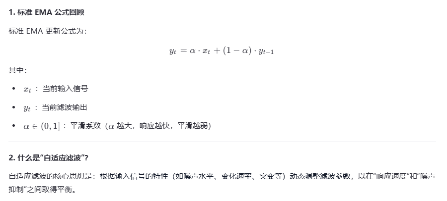
EMA（Exponential Moving Average，指数移动平均）本身是一种轻量级的低通滤波器，常用于平滑时间序列数据。虽然它不是传统意义上的“自适应滤波器”（如 LMS、RLS 等），但可以通过让 EMA 的平滑系数（通常记为 α ）动态调整，使其具备自适应性，从而实现一种简单的自适应滤波。

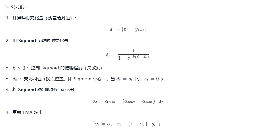
“根据信号变化率自适应调整 EMA 平滑系数 α，使用 Sigmoid 型函数” 的实现方法，并附上清晰的公式推导、参数解释和 Python 代码示例

调参技巧

1.先固定 αmin​,αmax​ ，调 d0​ 和 k

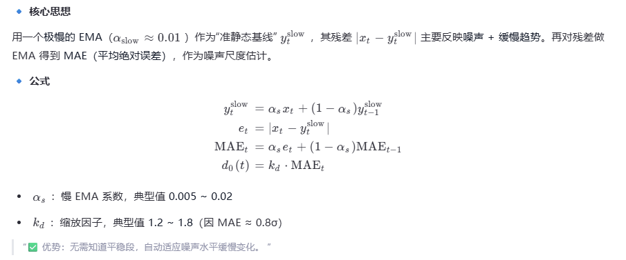
离线估计噪声标准差：

def estimate_d0_offline(signal, N0=100, c=2.0):
    """
    从信号前 N0 个点估计噪声标准差，计算 d0
    """
    sigma = np.std(signal[:N0])
    return c * sigma

在线估计：

下面给出Python 示例代码仅供参考，可根据需要自行调整参数

import numpy as np
import matplotlib.pyplot as plt

# 中文显示标题
plt.rcParams['font.sans-serif'] = ['SimHei']


class EMAFilter:
    """指数移动平均滤波器"""

    def __init__(self, alpha=0.3):
        """
        初始化滤波器
        :param alpha: 平滑系数（0 < alpha < 1），值越大响应越快，平滑性越差
        """
        self.alpha = alpha
        self.last_output = None  # 保存上一时刻的滤波结果

    def filter(self, x):
        """
        对单个数据点进行滤波
        :param x: 当前输入数据
        :return: 滤波后的数据
        """
        if self.last_output is None:
            # 首次输入时，直接将输入作为初始输出
            self.last_output = x
        else:
            # EMA核心公式：当前输出 =  alpha*当前输入 + (1-alpha)*上一时刻输出
            self.last_output = self.alpha * x + (1 - self.alpha) * self.last_output
        return self.last_output

    def reset(self):
        """重置滤波器状态"""
        self.last_output = None


class OnlineD0Estimator:
    def __init__(self, alpha_slow=0.01, k_d=1.5):
        self.alpha_slow = alpha_slow
        self.k_d = k_d
        self.y_slow = None  # 慢速基线
        self.mae = None  # 噪声尺度估计（MAE）

    def update(self, x):
        if self.y_slow is None:
            self.y_slow = x
            self.mae = 0.0
            return self.k_d * self.mae  # 初始 d0 = 0

        # 更新慢速基线
        self.y_slow = self.alpha_slow * x + (1 - self.alpha_slow) * self.y_slow
        # 计算残差绝对值
        err = abs(x - self.y_slow)
        # 更新 MAE（噪声尺度）
        self.mae = self.alpha_slow * err + (1 - self.alpha_slow) * self.mae
        # 返回 d0
        return self.k_d * self.mae


class FullyAdaptiveEMA:
    def __init__(self, alpha_min=0.02, alpha_max=0.6, k_sigmoid=12.0):
        self.alpha_min = alpha_min
        self.alpha_max = alpha_max
        self.k_sigmoid = k_sigmoid
        self.y = None

        # 在线 d0 估计器
        self.d0_estimator = OnlineD0Estimator(alpha_slow=0.01, k_d=1.5)

    def update(self, x):
        # 实时估计 d0
        d0 = self.d0_estimator.update(x)

        if self.y is None:
            self.y = x
            return self.y

        # 计算残差
        d = abs(x - self.y)
        # Sigmoid 映射
        s = 1.0 / (1.0 + np.exp(-self.k_sigmoid * (d - d0 + 1e-8)))  # +eps 防 d0=0
        alpha = self.alpha_min + (self.alpha_max - self.alpha_min) * s
        # 更新输出
        self.y = alpha * x + (1 - alpha) * self.y
        return self.y


# 生成测试数据（含噪声的正弦波）
def generate_test_data():
    # 生成时间序列（0到10秒，共1000个点）
    t = np.linspace(0, 10, 1000)
    # 原始信号（正弦波）
    signal = np.sin(t)
    # 添加高斯噪声（均值0，标准差0.5）
    noise = np.random.normal(0, 0.5, size=len(t))
    noisy_signal = signal + noise
    return t, signal, noisy_signal


# 主函数：测试不同alpha的滤波效果
def main():
    # 生成测试数据
    t, original_signal, noisy_signal = generate_test_data()

    # 初始化滤波器
    ema_fixed_low = EMAFilter(alpha=0.05)  # 强平滑
    ema_fixed_high = EMAFilter(alpha=0.3)  # 快响应
    ema_adaptive = FullyAdaptiveEMA(alpha_min=0.02, alpha_max=0.6, k_sigmoid=12.0)

    # 存储滤波结果
    filtered_low = []
    filtered_high = []
    filtered_adaptive = []

    # 逐点滤波
    for x in noisy_signal:
        filtered_low.append(ema_fixed_low.filter(x))
        filtered_high.append(ema_fixed_high.filter(x))
        filtered_adaptive.append(ema_adaptive.update(x))

    # 转换为numpy数组
    filtered_low = np.array(filtered_low)
    filtered_high = np.array(filtered_high)
    filtered_adaptive = np.array(filtered_adaptive)

    # 计算RMSE（均方根误差）作为客观评价指标
    rmse_low = np.sqrt(np.mean((filtered_low - original_signal) ** 2))
    rmse_high = np.sqrt(np.mean((filtered_high - original_signal) ** 2))
    rmse_adaptive = np.sqrt(np.mean((filtered_adaptive - original_signal) ** 2))

    # 绘图
    plt.figure(figsize=(14, 8))

    plt.plot(t, noisy_signal, 'lightgray', alpha=0.7, linewidth=1, label='含噪声信号')
    plt.plot(t, original_signal, 'k--', linewidth=2, label='原始信号')
    plt.plot(t, filtered_low, 'b-', linewidth=2, label=f'固定α=0.05 (RMSE={rmse_low:.3f})')
    plt.plot(t, filtered_high, 'g-', linewidth=2, label=f'固定α=0.3 (RMSE={rmse_high:.3f})')
    plt.plot(t, filtered_adaptive, 'r-', linewidth=2.5, label=f'自适应α (RMSE={rmse_adaptive:.3f})')

    plt.xlabel('时间')
    plt.ylabel('幅值')
    plt.title('固定α vs 自适应α EMA滤波效果对比')
    plt.legend()
    plt.grid(True, alpha=0.3)
    plt.tight_layout()
    plt.show()

    # 打印客观指标
    print(f"RMSE 比较:")
    print(f"  固定α=0.05: {rmse_low:.4f}")
    print(f"  固定α=0.3:   {rmse_high:.4f}")
    print(f"  自适应α:     {rmse_adaptive:.4f}")

    return t, original_signal, noisy_signal, filtered_low, filtered_high, filtered_adaptive


# 运行主函数
if __name__ == "__main__":
    results = main()