About Backpropagation (反向传播法）

最新推荐文章于 2024-10-03 03:54:06 发布

数据架构

最新推荐文章于 2024-10-03 03:54:06 发布

阅读量261

点赞数

分类专栏： Python learning 文章标签：深度学习神经网络人工智能

本文链接：https://blog.youkuaiyun.com/u011868279/article/details/125365337

版权

Python learning 专栏收录该内容

33 篇文章

订阅专栏

这篇教程详细介绍了反向传播算法在多层感知机中的应用，从初始化网络、正向传播、反向传播错误、训练网络到预测输出的全过程。使用了一个简单的神经网络结构，通过模拟数据进行训练，并展示了如何在小麦种子分类问题上应用这些概念。此外，还提供了完整的Python代码示例，便于读者理解并实践。

摘要生成于 C知道，由 DeepSeek-R1 满血版支持，前往体验 >

The backpropagation is the classical feedforward artificial neural network. It is used to train large deep learning networks.

After this part, you will know:

How to forward-propagate(正向传播) an input to calculate an output
How to backpropagate(反向传播) error and train a network
How to apply the backpropagation algorithm to a real-world predictive modeling problem.

1.1 Description

A brief introduction to the Backpropagation Algorithm
The Wheat Seeds dataset

1.1.1 Backpropagation Algorithm

The Backpropagation algorithm is a supervised learning method for multilayer feedforward networks from the field of Artificial Neural Networks. Feedforward neural networks are inspired by the information processing of one or more neural cells.called a neuron.

The principle of the backpropagation approach is to model a given function by modifying internal weightings of input signals to produce an expected output signal. The backpropagation algorithm is a method for training the weights in a multilayer feedforward neural network.

A standard network structure :

input layer
hidden layer
output layer

Backpropagation can be used for both classification and regression problems.

1.1.2 Wheat Seeds Dataset

This dataset involves the prediction of the species of wheat seeds . The baseline performance on the problem is approximately 28% . the filename seeds_dataset.csv. The dataset is in tab-separated format, so must convert it to CSV using a text editior or a spreadsheet program.

1.2 Tutorial

This tutorial is broken down into 6 parts:

Initialize Network
Forward-Propagate
Backpropagate Error
Train Network
Predict
Wheat Seeds Case Study

1.2.1 Initialize Network

the creation of a new network ready for training. Each neuron has a set of weights that need to be maintained. One weight for each input connection and an additional weights for the bias.use a dictionary to represent each neuron and store properties.

Below is a function named initialize_network() that creates a new neural network ready for training.

accpet three parameters:

the number of inputs
the number of neurons to have in the hidden layer
the number of outputs

# Function to Initialize a Multilayer Perceptron Network
# Initialize a network
def initialize_network(n_inputs, n_hidden, n_outputs):
    network = list()
    hidden_layer = [{'weights':[random() for i in range(n_inputs + 1)]} for i in range(n_hidden)]
    network.append(hidden_layer)
    output_layer = [{'weights':[random() for i in range(n_hidden + 1)]} for i in range(n_outputs)]
    network.append(output_layer)
    return network

Below is a complete example that creates a small network.

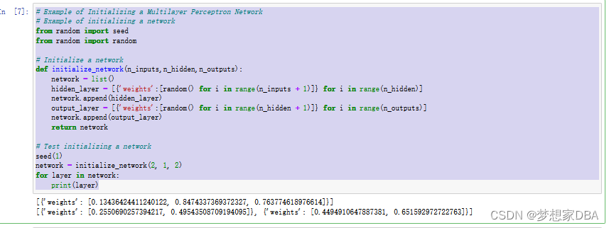
# Example of Initializing a Multilayer Perceptron Network
# Example of initializing a network
from random import seed
from random import random

# Initialize a network
def initialize_network(n_inputs,n_hidden,n_outputs):
    network = list()
    hidden_layer = [{'weights':[random() for i in range(n_inputs + 1)]} for i in range(n_hidden)]
    network.append(hidden_layer)
    output_layer = [{'weights':[random() for i in range(n_hidden + 1)]} for i in range(n_outputs)]
    network.append(output_layer)
    return network

# Test initializing a network
seed(1)
network = initialize_network(2, 1, 2)
for layer in network:
    print(layer)

Running the example, you can see that the code prints out each layer one by one. You can see the hidden layer has one neuron with 2 input weights plus the bias. The output layer has 2 neurons, each with 1 weight plus the bias.

1.2.2 Forward-Propagate

We can break-propagation down into three parts:

Neuron Activation
Neuron Transfer
Forward-Propagation

Neuron Activation

Neuron activation is calculated as the weighted sum of the inputs.Much like linear regression.

$activation = bias + \sum_{i=1}^{n}weight_{i}\times input_{i}$

weight is a network weight

input is an input value

i is the index of a weight or an input

bias is a special weight that has no input to multiply with .

Below is an implementation of this in a function named activate()

# Calculate neuron activation for an input
def activate(weights, inputs):
    activation = weights[-1]
    for i in range(len(weights)-1):
        activation += weights[i] * inputs[i]
    return activation

How to use the neuron activation

Neuron Transfer

Once a neuron is actived,we need to transfer the activation to see what the neuron output actually is .

Different transfer functions can be used.

It is traditional to use the sigmod activation function
use the tanh(hyperbolic tangent) function to transfer outputs.

we can transfer an activation function using the sigmoid function as follows:

where e is the base of the natural logarithms(Euler's number).Below is a function named transfer() that implements the sigmoid equation.

# Transfer neuron activation
def transfer(activation):
    return 1.0 / (1.0 + exp(-activation))

Forward-Propagation

Forward-propagating an input is straightforward.Below is a function named forward_propagate() that implement the forwarding-propagation for a row data from our dataset with our neural network.The function returns the outputs from the last layer also called the output layer.

# Forward-propagate input to a network output
def forward_propagate(network, row):
    inputs = row
    for layer in network:
        new_inputs = []
        for neuron in layer:
            activation = activate(neuron['weights'],inputs)
            neuron['output'] = transfer(activation)
            new_inputs.append(neuron['output'])
        inputs = new_inputs
    return inputs

# Example of Forward-Propagating an Input Through a Network
# Example of forward propagating input
from math import exp

# Calculate neuron activation for an input
def activate(weights,inputs):
    activation = weights[-1]
    for i in range(len(weights)-1):
        activation += weights[i] * inputs[i]
    return activation

# Transfer neuron activation
def transfer(activation):
    return 1.0 / (1.0 + exp(-activation))

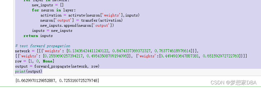
# Forward propagate input to a network output
def forward_propagate(network, row):
    inputs = row
    for layer in network:
        new_inputs = []
        for neuron in layer:
            activation = activate(neuron['weights'],inputs)
            neuron['output'] = transfer(activation)
            new_inputs.append(neuron['output'])
        inputs = new_inputs
    return inputs

# test forward propagation
network = [[{'weights': [0.13436424411240122, 0.8474337369372327, 0.763774618976614]}],
[{'weights': [0.2550690257394217, 0.49543508709194095]}, {'weights':[0.4494910647887381, 0.651592972722763]}]]
row = [1, 0, None]
output = forward_propagate(network, row)
print(output)

Sample Output from Forward-Propagate Input Through a Network.

1.2.3 Backpropagate Error

Transfer Derivative
Error Backpropagation

Transfer Derivative

Given an output value from a neuron, we need to calculate it's slope.We are using the sigmoid transfer function, the derivative of which can be calculated as follows:

$derivative = output \times (1.0 - output)$

Error Backpropagation

$error = (expected - output)\times transfer\_derivative(output)$

expected is the expected output value for the neuron, output is the output value for the neuron and transfer_derivative() calculates the slope of the neuron's output layer.The expected value is the class value itself.

The backpropagated error signal is accumulated and then used to determine the error for the neuron in the hidden layer.as follows:

$error = (weight_{k}\times error_{j})\times transfer_derivative(output)$

$error_{j}$ is the error signal from the jth neuron in the output layer.

$weight_{k}$ is the weight that connects the kth neuron to the current and output is the output for the current neuron.

Below is a function backward_propagate_error() that implements this procedure.

# Backpropagate error and store in neurons
def backward_propagate_error(network, expected):
    for i in reversed(range(len(network))):
        layer = network[i]
        errors = list()
        if i != len(network)-1:
            for j in range(len(layer)):
                error = 0.0
                for neuron in network[i + 1]:
                    error += (neuron['weights'][j] * neuron['delta'])
                errors.append(error)
        else:
            for j in range(len(layer)):
                neuron = layer[j]
                errors.append(expected[j] - neuron['output'])
            for j in range(len(layer)):
                neuron = layer[j]
                neuron['delta'] = errors[j] * transfer_derivative(neuron['output'])

we define a fixed neural network with output values and backpropagate an expected output pattern. The complete example is listed below:

# Example of backpropagating error

# Calculate the derivative of an neuron output
def transfer_derivative(output):
    return output * (1.0 - output)

# Backpropagate error and store in neurons
def backward_propagate_error(network,expected):
    for i in reversed(range(len(network))):
        layer = network[i]
        errors = list()
        if i != len(network)-1:
            for j in range(len(layer)):
                error = 0.0
                for neuron in network[i + 1]:
                    error += (neuron['weights'][j]*neuron['delta'])
                errors.append(error)
        else:
            for j in range(len(layer)):
                neuron = layer[j]
                errors.append(expected[j] - neuron['output'])
        for j in range(len(layer)):
            neuron = layer[j]
            neuron['delta'] = errors[j] * transfer_derivative(neuron['output'])

# test backpropagation of error
network = [[{'output': 0.7105668883115941, 'weights': [0.13436424411240122,0.8474337369372327, 0.763774618976614]}],
[{'output': 0.6213859615555266, 'weights': [0.2550690257394217, 0.49543508709194095]},
{'output': 0.6573693455986976, 'weights': [0.4494910647887381, 0.651592972722763]}]]

expected = [0, 1]
backward_propagate_error(network, expected)
for layer in network:
    print(layer)

1.2.4 Train Network

Update Weights
Train Network

Update Weights

Network weights are updated as follows:

$weight = weight + learning\_rate \times error \times input$

weight is a given weight

learning_rate is a parameter that you must specify

error is the error calculated by the backpropagation procedure for the neuron

input is the input value that caused the error.

Below is a function named update_weights() that updates the weights for a network given an input row of data.

# Update network weights with error
def update_weights(network,row,l_rate):
    for i in range(len(network)):
        inputs = row[:-1]
        if i != 0:
            inputs = [neuron['output'] for neuron in network[i-1]]
        for neuron in network[i]:
            for j in range(len(inputs)):
                neuron['weights'][j] += l_rate * neuron['delta'] * inputs[j]
            neuron['weights'][-1] += l_rate * neuron['delta']

Train Network

# Train a network for a fixed number of epochs
def train_network(network, train, l_rate, n_epoch,n_outputs):
    for epoch in range(n_epoch):
        sum_error = 0
        for row in train:
            outputs = forward_propagate(network,row)
            expected = [0 for i in range(n_outputs)]
            expected[row[-1]] = 1
            sum_error += sum([(expected[i]-output[i])**2 for i in range(len(expected))])
            backward_propagate_error(network,expected)
            update_weights(network,row,l_rate)
        print('>epoch=%d, lrate=%.3f, error=%.3f' % (epoch, l_rate,sum_error))

Below is a small contrived dataset that we can use to test out training our neural network.

X1            X2             Y
2.7810836     2.550537003    0
1.465489372   2.362125076    0
3.396561688   4.400293529    0
1.38807019    1.850220317    0
3.06407232    3.005305973    0
7.627531214   2.759262235    1
5.332441248   2.088626775    1
6.922596716   1.77106367     1
8.675418651   -0.242068655   1
7.673756466   3.508563011    1

# Example of training a network by backpropagation
from math import exp
from random import seed
from random import random

# Initialize a network
def initialize_network(n_inputs, n_hidden,n_outputs):
    network = list()
    hidden_layer = [{'weights':[random() for i in range(n_inputs + 1)]} for i in range(n_hidden)]
    network.append(hidden_layer)
    output_layer = [{'weights':[random() for i in range(n_hidden+ 1)]} for i in range(n_outputs)]
    network.append(output_layer)
    return network

# Calculate neuron activation for an input
def activate(weights, inputs):
    activation = weights[-1]
    for i in range(len(weights)-1):
        activation += weights[i] * inputs[i]
    return activation

# Transfer neuron activation
def transfer(activation):
    return 1.0/ (1.0 + exp(-activation))

# Forward propgate input to a network output
def forward_propagate(network, row):
    inputs = row
    for layer in network:
        new_inputs = []
        for neuron in layer:
            activation = activate(neuron['weights'],inputs)
            neuron['output'] = transfer(activation)
            new_inputs.append(neuron['output'])
        inputs = new_inputs
    return inputs

# Calculate the derivative of an neuron output
def transfer_derivative(output):
    return output * (1.0 - output)

# Backpropagate error and store in neurons
def backward_propagate_error(network,expected):
    for i in reversed(range(len(network))):
        layer = network[i]
        errors = list()
        if i != len(network)-1:
            for j in range(len(layer)):
                error = 0.0
                for neuron in network[i+1]:
                    error += (neuron['weights'][j] * neuron['delta'])
                errors.append(error)
        else:
            for j in range(len(layer)):
                neuron = layer[j]
                errors.append(expected[j] - neuron['output'])
        for j in range(len(layer)):
            neuron = layer[j]
            neuron['delta'] = errors[j]* transfer_derivative(neuron['output'])

# Update network weights with error
def update_weights(network, row, l_rate):
    for i in range(len(network)):
        inputs = row[:-1]
        if i != 0:
            inputs = [neuron['output'] for neuron in network[i - 1]]
        for neuron in network[i]:
            for j in range(len(inputs)):
                neuron['weights'][j] += l_rate * neuron['delta'] * inputs[j]
            neuron['weights'][-1] += l_rate * neuron['delta']
            
# Train a network for a fixed number of epochs
def train_network(network, train, l_rate, n_epoch,n_outputs):
    for epoch in range(n_epoch):
        sum_error = 0
        for row in train:
            outputs = forward_propagate(network, row)
            expected = [0 for i in range(n_outputs)]
            expected[row[-1]] = 1
            sum_error += sum([(expected[i]-outputs[i])**2 for i in range(len(expected))])
            backward_propagate_error(network,expected)
            update_weights(network,row,l_rate)
        print('>epoch=%d, lrate=%.3f, error=%.3f' % (epoch, l_rate, sum_error))
        
# Test training backprop algorithm
seed(1)
dataset = [[2.7810836,2.550537003,0],
[1.465489372,2.362125076,0],
[3.396561688,4.400293529,0],
[1.38807019,1.850220317,0],
[3.06407232,3.005305973,0],
[7.627531214,2.759262235,1],
[5.332441248,2.088626775,1],
[6.922596716,1.77106367,1],
[8.675418651,-0.242068655,1],
[7.673756466,3.508563011,1]]

n_inputs = len(dataset[0]) - 1
n_outputs = len(set([row[-1] for row in dataset]))
network = initialize_network(n_inputs,2,n_outputs)
train_network(network,dataset, 0.5,20,n_outputs)
for layer in network:
    print(layer)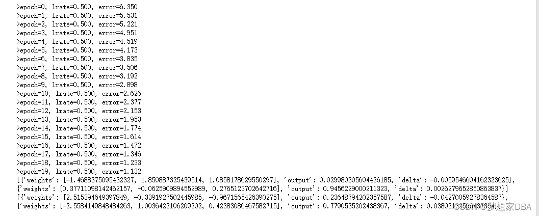

1.2.5 Predict

Below is a function named predict() that implements this procedure.

# Make a prediction with a network
def predict(network, row):
    outputs = forward_propagate(network,row)
    return outputs.index(max(outputs))

The complete example is listed below:

# Example of making predictions
from math import exp

# Calculate neuron activation for an input
def activate(weights,inputs):
    activation = weights[-1]
    for i in range(len(weights)-1):
        activation += weights[i] * inputs[i]
    return activation
# Transfer neuron activation
def transfer(activation):
    return 1.0 / (1.0 + exp(-activation))

# Forward propagate input to a network output
def forward_propagate(network, row):
    inputs = row
    for layer in network:
        new_inputs = []
        for neuron in layer:
            activation = activate(neuron['weights'],inputs)
            neuron['output'] = transfer(activation)
            new_inputs.append(neuron['output'])
        inputs = new_inputs
    return inputs

# Make a prediction with a network
def predict(network, row):
    outputs = forward_propagate(network, row)
    return outputs.index(max(outputs))

# Test making predictions with the network
dataset = [[2.7810836,2.550537003,0],
[1.465489372,2.362125076,0],
[3.396561688,4.400293529,0],
[1.38807019,1.850220317,0],
[3.06407232,3.005305973,0],
[7.627531214,2.759262235,1],
[5.332441248,2.088626775,1],
[6.922596716,1.77106367,1],
[8.675418651,-0.242068655,1],
[7.673756466,3.508563011,1]]
network = [[{'weights': [-1.482313569067226, 1.8308790073202204, 1.078381922048799]},{'weights': [0.23244990332399884, 0.3621998343835864, 0.40289821191094327]}],
[{'weights': [2.5001872433501404, 0.7887233511355132, -1.1026649757805829]}, {'weights':[-2.429350576245497, 0.8357651039198697, 1.0699217181280656]}]]
for row in dataset:
    prediction = predict(network, row)
    print('Expected=%d, Got=%d' % (row[-1], prediction))

1.2.6 Wheat Seeds Case Study

load_csv() to load the file

str_column_to_float() to convert string numbers to floats

str_column_to_int() to convert the class column to integer values

evaluate_algorithm() to evaluate the algorithm with cross-validation

accuracy_metric() to calculate the accuracy of predictions

back_propagation() was developed to manage the application of the Backpropagation algorithm,first initializing a network,training it on the training dataset and then using the trained network to make predictions on a test dataset.

The complete example is listed below:

# Backprop on the Seeds Dataset
from random import seed
from random import randrange
from random import random
from csv import reader
from math import exp

# Load a CSV file
def load_csv(filename):
    dataset = list()
    with open(filename,'r') as file:
        csv_reader = reader(file)
        for row in csv_reader:
            if not row:
                continue
            dataset.append(row)
    return dataset

# Convert string column to float
def str_column_to_float(dataset, column):
    for row in dataset:
        row[column] = float(row[column].strip())
        
# Convert string column to integer
def str_column_to_int(dataset, column):
    class_values = [row[column] for row in dataset]
    unique = set(class_values)
    lookup = dict()
    for i,value in enumerate(unique):
        lookup[value] = i
    for row in dataset:
        row[column] = lookup[row[column]]
    return lookup

# Find the min and max values for each column
def dataset_minmax(dataset):
    return [[min(column),max(column)] for column in zip(*dataset)]

# Rescale dataset columns to the range 0 - 1
def normalize_dataset(dataset, minmax):
    for row in dataset:
        for i in range(len(row)-1):
            row[i] = (row[i] - minmax[i][0]) / (minmax[i][1] - minmax[i][0])

# Split a dataset into k folds
def cross_validation_split(dataset, n_folds):
    dataset_split = list()
    dataset_copy = list(dataset)
    fold_size = int(len(dataset) / n_folds)
    for i in range(n_folds):
        fold = list()
        while len(fold) < fold_size:
            index = randrange(len(dataset_copy))
            fold.append(dataset_copy.pop(index))
        dataset_split.append(fold)
    return dataset_split

# Calculate accuracy percentage
def accuracy_metric(actual,predicted):
    correct = 0
    for i in range(len(actual)):
        if actual[i] == predicted[i]:
            correct += 1
        return correct / float(len(actual)) * 100.0
    
# Evaluate an algorithm using a cross validation split
def evaluate_algorithm(dataset, algorithm,n_folds,*args):
    folds = cross_validation_split(dataset,n_folds)
    scores = list()
    for fold in folds:
        train_set = list(folds)
        train_set.remove(fold)
        train_set = sum(train_set,[])
        test_set = list()
        for row in fold:
            row_copy = list(row)
            test_set.append(row_copy)
            row_copy[-1] = None
        predicted = algorithm(train_set, test_set, *args)
        actual = [row[-1] for row in fold]
        accuracy = accuracy_metric(actual,predicted)
        scores.append(accuracy)
    return scores

# Calculate neuron activation for an input
def activate(weights, inputs):
    activation = weights[-1]
    for i in range(len(weights)-1):
        activation += weights[i] * input[i]
    return activation

# Transfer neuron activation
def transfer(activation):
    return 1.0 / (1.0 + exp(-activation))

# Forward propagate input to a network output
def forward_propagate(network,row):
    inputs = row
    for layer in network:
        new_inputs = []
        for neuron in layer:
            activation = activate(neuron['weights'],inputs)
            neuron['output'] = transfer(activation)
            new_inputs.append(neuron['output'])
        inputs = new_inputs
    return inputs

# Backpropagate error and store in enurons
def backward_propagate_error(network, expected):
    for i in reversed(range(len(network))):
        layer = network[i]
        errors = list()
        if i != len(network)-1:
            for j in range(len(layer)):
                error = 0.0
                for neuron in network[i + 1]:
                    error += (neuron['weights'][j]*neuron['delta'])
                errors.append(error)
        else:
            for j in range(len(layer)):
                neuron = layer[j]
                errors.append(expected[j] - neuron['output'])
        for j in range(len(layer)):
            neuron = layer[j]
            neuron['delta'] = errors[j] * transfer_derivative(neuron['output'])
            
# Update network weights with error
def update_weights(network,row,l_rate):
    for i in range(len(network)):
        inputs = row[:-1]
        if i != 0:
            inputs = [neuron['output'] for neuron in network[i-1]]
        for neuron in network[i]:
            for j in range(len(inputs)):
                neuron['weights'][j] += l_rate * enuron['delta'] * input[j]
                neuron['weights'][-1]+= l_rate * enuron['delta']
                
# Train a network for a fixed number of epochs
def train_network(network, train,l_rate,n_epoch,n_outputs):
    for i in range(n_epoch):
        for row in train:
            forward_propagate(network,row)
            expected = [0 for i in range(n_outputs)]
            expected[row[-1]] = 1
            backward_propagate_error(network, expected)
            update_weights(network,row,l_rate)
            
# Initialize a network
def initialize_network(n_inputs,n_hidden,n_outputs):
    network = list()
    hidden_layer = [{'weights':[random() for i in range(n_inputs + 1)]} for i in range(n_hidden)]
    network.append(hidden_layer)
    output_layer = [{'weights':[random() for i in range(n_hidden + 1)]} for i in range(n_outputs)]
    network.append(output_layer)
    return network

# Make a prediction with a network
def predict(network, row):
    outputs = forward_propagate(network,row)
    return outputs.index(max(outputs))

# Backpropagation Algorithm with Stochastic Gradient Descent
def back_propagation(train,test,l_rate,n_epoch,n_hidden):
    n_inputs = len(train[0]) -1
    n_outputs = len(set([row[-1] for row in train]))
    network = initialize_network(n_inputs,n_hidden,n_outputs)
    train_network(network, train, l_rate, n_epoch, n_outputs)
    predictions = list()
    for row in test:
        prediction = predict(network,row)
        predictions.append(prediction)
    return (predictions)

# Test Backprop on Seed dataset
seed(1)
# load and prepare data
filename = 'seeds_dataset.csv'
dataset = load_csv(filename)
for i in range(len(dataset[0])-1):
    str_column_to_float(dataset,i)
# convert class column to integers
str_column_to_int(dataset,len(dataset[0])-1)
# normalize input variances
minmax = dataset_minmax(dataset)
normalize_dataset(dataset,minmax)
# evaluate algorithm
n_folds = 5
l_rate = 0.3
n_epoch = 500
n_hidden = 5
scores = evaluate_algorithm(dataset, back_propagation, n_folds, l_rate, n_epoch, n_hidden)
print('Scores: %s' % scores)
print('Mean Accuracy: %.3f%%' % (sum(scores)/float(len(scores))))