How to work through Regression Machine Learning Case Study Project

数据架构

已于 2022-05-30 15:38:13 修改

阅读量238

点赞数

分类专栏： Machine Learning 文章标签：机器学习深度学习人工智能

于 2022-05-30 15:36:37 首次发布

本文链接：https://blog.youkuaiyun.com/u011868279/article/details/125039585

版权

Machine Learning 专栏收录该内容

35 篇文章

订阅专栏

How do you work through a predictive modeling machine learning problem end-to-end? In this lesson you will work through a case study regression predictive modeling problem in Python including each step of the applied machine learning process. After completing this project, you will know:

How to work through a regression predictive modeling problem end-to-end.
How to use data transforms to improve model performance.
How to use algorithm tuning to improve model performance.
How to use ensemble methods and tuning of ensemble methods to improve model performance.

1.1 Problem Definition

For this project we will investigate the Boston House Price dataset. Each record in the database describes a Boston suburb or town. The data was drawn from the Boston Standard Metropolitan Statistical Area (SMSA) in 1970. The attributes are defined as follows (taken from the UCI Machine Learning Repository ):

CRIM: per capita crime rate by town
ZN: proportion of residential land zoned for lots over 25,000 sq.ft.
INDUS: proportion of non-retail business acres per town
CHAS: Charles River dummy variable (= 1 if tract bounds river; 0 otherwise)
NOX: nitric oxides concentration (parts per 10 million)
RM: average number of rooms per dwelling
AGE: proportion of owner-occupied units built prior to 1940
DIS: weighted distances to five Boston employment centers
RAD: index of accessibility to radial highways
TAX: full-value property-tax rate per $10,000
PTRATIO: pupil-teacher ratio by town
B: 1000(Bk − 0.63)2 where Bk is the proportion of blacks by town
LSTAT: % lower status of the population
MEDV: Median value of owner-occupied homes in $1000s

1.2 Load the Dataset

Let’s start off by loading the libraries required for this project.

# Load libraries
import numpy as np
from numpy import arange
from matplotlib import pyplot
from pandas import read_csv
from pandas import set_option
from pandas.plotting import scatter_matrix
from sklearn.preprocessing import StandardScaler
from sklearn.model_selection import train_test_split
from sklearn.model_selection import KFold
from sklearn.model_selection import cross_val_score
from sklearn.model_selection import GridSearchCV
from sklearn.linear_model import LinearRegression
from sklearn.linear_model import Lasso
from sklearn.linear_model import ElasticNet
from sklearn.tree import DecisionTreeRegressor
from sklearn.neighbors import KNeighborsRegressor
from sklearn.svm import SVR
from sklearn.pipeline import Pipeline
from sklearn.ensemble import RandomForestRegressor
from sklearn.ensemble import GradientBoostingRegressor
from sklearn.ensemble import ExtraTreesRegressor
from sklearn.ensemble import AdaBoostRegressor
from sklearn.metrics import mean_squared_error

We can now load the dataset that you can download from the UCI Machine Learning repository website.

# Load dataset
filename = 'housing.csv'
names = ['CRIM','ZN','INDUS','CHAS','NOX','RM','AGE','DIS','RAD','TAX','PTRATIO','B','LSTAT','MEDV']
dataset = read_csv(filename, names=names)

You can see that we are specifying the short names for each attribute so that we can reference them clearly later. we indicate this to read_csv() function . We now have our data loaded.

1.3 Analyze Data

We can now take a closer look at our loaded data.

1.3.1 Descriptive Statistics

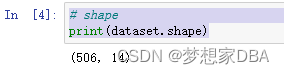
Let's start off by confirming the dimension of the dataset, the number of rows and columns.

# shape
print(dataset.shape)

We have 506 instances to work with and can confirm the data has 14 attributes including the output attribute MEDV.

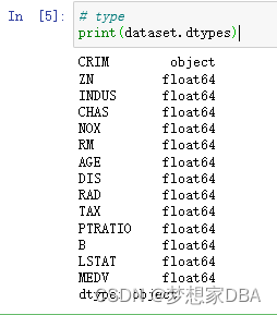
Let's also look at the data types of each attribute.

# type 
print(dataset.dtypes)

We can see that all of the attributes are numeric, mostly real values (float) and some have been interpreted as integers (int).

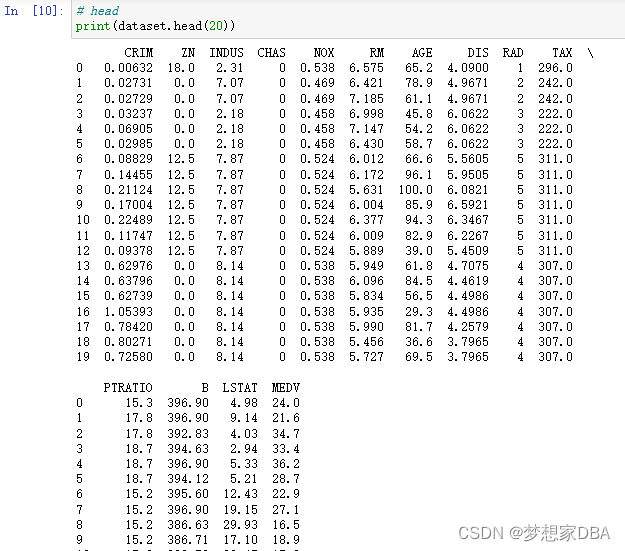
Let’s now take a peek at the first 20 rows of the data.

Let’s summarize the distribution of each attribute.

# descriptions
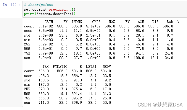
set_option('precision',1)
print(dataset.describe())

We now have a better feeling for how different the attributes are. The min and max values as well are the means vary a lot. We are likely going to get better results by rescaling the data in some way.

Now, let’s now take a look at the correlation between all of the numeric attributes.

# correlation
set_option('precision', 2)
print(dataset.corr(method='pearson'))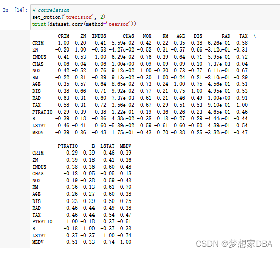

1.4 Data Visualizations

1.4.1 Unimodal Data Visualizations

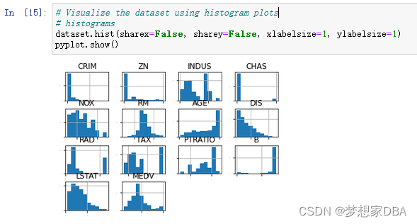
Let’s look at visualizations of individual attributes. It is often useful to look at your data using multiple different visualizations in order to spark ideas. Let’s look at histograms of each attribute to get a sense of the data distributions.

# Visualize the dataset using histogram plots
# histograms
dataset.hist(sharex=False, sharey=False, xlabelsize=1, ylabelsize=1)
pyplot.show()

We can see that some attributes may have an exponential distribution, such as CRIM, ZN, AGE and B. We can see that others may have a bimodal distribution such as RAD and TAX.

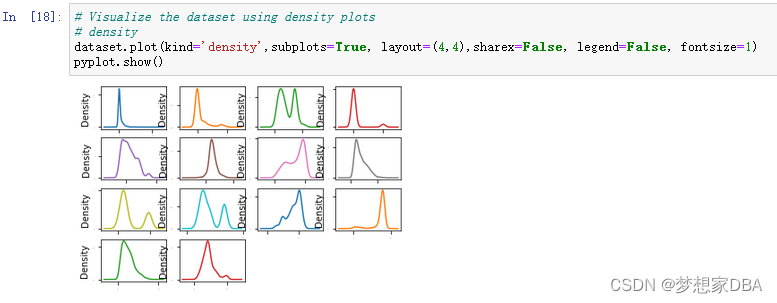
Let’s look at the same distributions using density plots that smooth them out a bit.

# Visualize the dataset using density plots
# density
dataset.plot(kind='density',subplots=True, layout=(4,4),sharex=False, legend=False, fontsize=1)
pyplot.show()

This perhaps adds more evidence to our suspicion about possible exponential and bimodal distributions. It also looks like NOX, RM and LSTAT may be skewed Gaussian distributions, which might be helpful later with transforms.

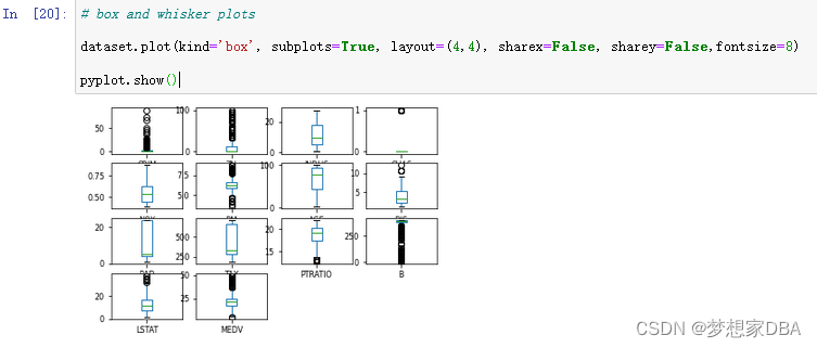
Let's look at the data with box and whisker plots of each attribute.

# box and whisker plots

dataset.plot(kind='box', subplot=True, layout=(4,4), sharex=False, sharey=False,fontsize=8)

pyplot.show()

This helps point out the skew in many distributions so much so that data looks like outliers (e.g. beyond the whisker of the plots).

1.4.2 Multimodal Data Visualizations

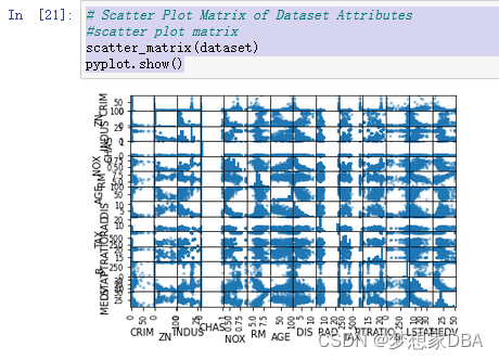
Let’s look at some visualizations of the interactions between variables. The best place to start is a scatter plot matrix.

# Scatter Plot Matrix of Dataset Attributes
#scatter plot matrix
scatter_matrix(dataset)
pyplot.show()

We can see that some of the higher correlated attributes do show good structure in their relationship. Not linear, but nice predictable curved relationships.

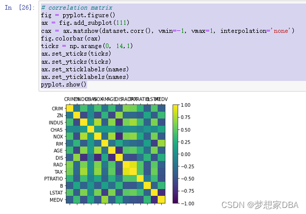
Let’s also visualize the correlations between the attributes.

# correlation matrix
fig = pyplot.figure()
ax = fig.add_subplot(111)
cax = ax.matshow(dataset.corr(), vmin=-1, vmax=1, interpolation='none')
fig.colorbar(cax)
ticks = np.arange(0, 14,1)
ax.set_xticks(ticks)
ax.set_yticks(ticks)
ax.set_xticklabels(names)
ax.set_yticklabels(names)
pyplot.show()

The dark red color shows positive correlation whereas the dark blue color shows negative correlation. We can also see some dark red and dark blue that suggest candidates for removal to better improve accuracy of models later on.

1.4.3 Summary of Ideas

There is a lot of structure in this dataset. We need to think about transforms that we could use later to better expose the structure which in turn may improve modeling accuracy. So far it would be worth trying:

Feature selection and removing the most correlated attributes.
Normalizing the dataset to reduce the effect of differing scales.
Standardizing the dataset to reduce the effects of differing distributions.

With lots of additional time I would also explore the possibility of binning (discretization) of the data. This can often improve accuracy for decision tree algorithms.

1.5 Validation Dataset

It is a good idea to use a validation hold-out set. This is a sample of the data that we hold back from our analysis and modeling. We use it right at the end of our project to confirm the accuracy of our final model. It is a smoke test that we can use to see if we messed up and to give us confidence on our estimates of accuracy on unseen data. We will use 80% of the dataset for modeling and hold back 20% for validation.

# Separate Data into a Training and Validation Datasets
# Split-out validation dataset
array = dataset.values
X = array[:,0:13]
Y = array[:, 13]
validation_size = 0.20
seed = 7
X_train,X_validation,Y_train,Y_validation = train_test_split(X,Y,test_size=validation_size,random_state=seed)

1.6 Evaluate Algorithms: Baseline

We have no idea what algorithms will do well on this problem. Gut feel suggests regression algorithms like Linear Regression and ElasticNet may do well. It is also possible that decision trees and even SVM may do well. I have no idea. Let’s design our test harness. We will use 10-fold cross validation. The dataset is not too small and this is a good standard test harness configuration. We will evaluate algorithms using the Mean Squared Error (MSE) metric. MSE will give a gross idea of how wrong all predictions are (0 is perfect).

# Configure Algorithm Evaluation Test Harness
# Test options and evaluation metric
num_folds = 10
seed = 7
scoring = 'neg_mean_squared_error'

Let’s create a baseline of performance on this problem and spot-check a number of different algorithms. We will select a suite of different algorithms capable of working on this regression problem. The six algorithms selected include:

Linear Algorithms: Linear Regression (LR), Lasso Regression (LASSO) and ElasticNet (EN).
Nonlinear Algorithms: Classification and Regression Trees (CART), Support Vector Regression (SVR) and k-Nearest Neighbors (KNN).

# Create the List of Algotithms to Evaluate
# Spot-Check Algorithms
models = []
models.append(('LR',LinearRegression()))
models.append(('LASSO',Lasso()))
models.append(('EN', ElasticNet()))
models.append(('KNN', KNeighborsRegressor()))
models.append(('CART',DecisionTreeRegressor()))
models.append(('SVR',SVR()))

The algorithms all use default tuning parameters. Let’s compare the algorithms. We will display the mean and standard deviation of MSE for each algorithm as we calculate it and collect the results for use later.

# Evaluate the List of Algorithms
# evaluate each model in turn
results = []
names = []
for name,model in models:
    kfold = KFold(n_splits=num_folds, random_state=seed, shuffle=True)
    cv_results = cross_val_score(model, X_train,Y_train,cv=kfold,scoring=scoring)
    results.append(cv_results)
    names.append(name)
    msg = "%s: %f (%f)" % (name, cv_results.mean(), cv_results.std())
    print(msg)

It looks like LR has the lowest MSE, followed closely by CART.

LR: -22.006009 (12.188886)
LASSO: -27.105803 (13.165915)
EN: -27.923014 (13.156405)
KNN: -39.808936 (16.507968)
CART: -26.232606 (16.441503)
SVR: -67.824705 (32.801530)

Let’s take a look at the distribution of scores across all cross validation folds by algorithm.

# Compare Algorithms
fig = pyplot.figure()
fig.suptitle('Algorithm Comparsion')
ax = fig.add_subplot(111)
pyplot.boxplot(results)
ax.set_xticklabels(names)
pyplot.show()

We can see similar distributions for the regression algorithms and perhaps a tighter distribution of scores for CART.

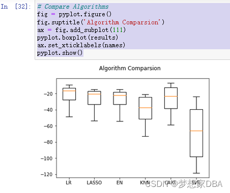
The differing scales of the data is probably hurting the skill of all of the algorithms and perhaps more so for SVR and KNN. In the next section we will look at running the same algorithms using a standardized copy of the data.

1.7 Evaluate Algorithms: Standardization

We suspect that the differing scales of the raw data may be negatively impacting the skill of some of the algorithms. Let’s evaluate the same algorithms with a standardized copy of the dataset. This is where the data is transformed such that each attribute has a mean value of zero and a standard deviation of 1. We also need to avoid data leakage when we transform the data. A good way to avoid leakage is to use pipelines that standardize the data and build the model for each fold in the cross validation test harness. That way we can get a fair estimation of how each model with standardized data might perform on unseen data.

# Standardize the dataset
pipelines = []
pipelines.append(('ScaledLR',Pipeline([('Scaler',StandardScaler()),('LR',LinearRegression())])))
pipelines.append(('ScaledLASSO', Pipeline([('Scaler', StandardScaler()),('EN',ElasticNet())])))
pipelines.append(('ScaledKNN', Pipeline([('Scaler', StandardScaler()),('KNN',KNeighborsRegressor())])))
pipelines.append(('ScaledCART', Pipeline([('Scaler', StandardScaler()),('CART',DecisionTreeRegressor())])))
pipelines.append(('ScaledSVR', Pipeline([('Scaler', StandardScaler()),('SVR',SVR())])))

results = []
names = []
for name, model in pipelines:
    kfold = KFold(n_splits=num_folds, random_state=seed, shuffle=True)
    cv_results = cross_val_score(model, X_train, Y_train, cv=kfold, scoring=scoring)
    results.append(cv_results)
    names.append(name)
    msg = "%s: %f (%f)" % (name, cv_results.mean(), cv_results.std())
    print(msg)

Running the example provides a list of mean squared errors. We can see that scaling did have an effect on KNN, driving the error lower than the other models.

ScaledLR: -22.006009 (12.188886)
ScaledLASSO: -28.301160 (13.609110)
ScaledKNN: -21.456867 (15.016218)
ScaledCART: -30.497448 (21.162739)
ScaledSVR: -29.570433 (18.052964)

Let’s take a look at the distribution of the scores across the cross validation folds.

# Compare Algorithms
fig = pyplot.figure()
fig.suptitle('Scaled Algorithm Comparsion')
ax = fig.add_subplot(111)
pyplot.boxplot(results)
ax.set_xticklabels(names)
pyplot.show()

We can see that KNN has both a tight distribution of error and has the lowest score.

1.8 Improve Results With Tuning

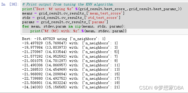
We know from the results in the previous section that KNN achieves good results on a scaled version of the dataset. But can it do better.The default value for the number of neighbors in KNN is 7. We can use a grid search to try a set of different numbers of neighbors and see if we can improve the score. The below example tries odd k values from 1 to 21, an arbitrary range covering a known good value of 7. Each k value(n_neighbors) is evaluated using 10-fold cross validation on a standardized copy of the training dataset.

# Tune the Parameters of the KNN Algorithm on the Standardized Dataset
# KNN Algorithm tuning
scaler = StandardScaler().fit(X_train)
rescaledX = scaler.transform(X_train)
k_values = np.array([1,3,5,7,9,11,13,15,17,19,21])
param_grid = dict(n_neighbors=k_values)
model = KNeighborsRegressor()
kfold = KFold(n_splits=num_folds, random_state=seed, shuffle=True)
grid = GridSearchCV(estimator=model, param_grid=param_grid,scoring=scoring,cv=kfold)
grid_result = grid.fit(rescaledX, Y_train)

We can display the mean and standard deviation scores as well as the best performing value for k below.

# Print output from tuning the KNN algorithm.
print("Best: %f using %s" %(grid_result.best_score_,grid_result.best_params_))
means = grid_result.cv_results_['mean_test_score']
stds = grid_result.cv_results_['std_test_score']
params = grid_result.cv_results_['params']
for mean, stdev,param in zip(means, stds, params):
    print("%f (%f) with: %r" %(mean, stdev, param))

You can see that the best for k (n neighbors) is 3 providing a mean squared error of -19.977984

, the best so far.

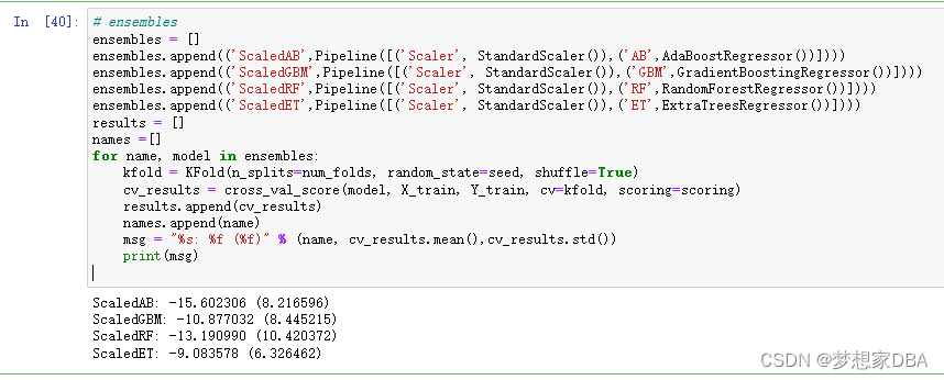
1.9 Ensemble Methods

Another way that we can improve the performance of algorithms on this problem is by using ensemble methods. In this section we will evaluate four different ensemble machine learning algorithms, two boosting and two bagging methods:

Boosting Methods: AdaBoost (AB) and Gradient Boosting (GBM).
Bagging Methods: Random Forests (RF) and Extra Trees (ET).

We will use the same test harness as before, 10-fold cross validation and pipelines that standardize the training data for each fold.

# ensembles
ensembles = []
ensembles.append(('ScaledAB',Pipeline([('Scaler', StandardScaler()),('AB',AdaBoostRegressor())])))
ensembles.append(('ScaledGBM',Pipeline([('Scaler', StandardScaler()),('GBM',GradientBoostingRegressor())])))
ensembles.append(('ScaledRF',Pipeline([('Scaler', StandardScaler()),('RF',RandomForestRegressor())])))
ensembles.append(('ScaledET',Pipeline([('Scaler', StandardScaler()),('ET',ExtraTreesRegressor())])))
results = []
names =[]
for name, model in ensembles:
    kfold = KFold(n_splits=num_folds, random_state=seed, shuffle=True)
    cv_results = cross_val_score(model, X_train, Y_train, cv=kfold, scoring=scoring)
    results.append(cv_results)
    names.append(name)
    msg = "%s: %f (%f)" % (name, cv_results.mean(),cv_results.std())
    print(msg)

Running the example calculates the mean squared error for each method using the default parameters. We can see that we’re generally getting better scores than our linear and nonlinear algorithms in previous sections.

We can also plot the distribution of scores across the cross validation folds.

# Visualzie the Differences in Ensemble Algorithm Performance on Standardized Dataset.
# Compare Algorithms
fig = pyplot.figure()
fig.suptitle('Scaled Ensemble Algorithm Comparison')
ax = fig.add_subplot(111)
pyplot.boxplot(results)
ax.set_xticklabels(names)
pyplot.show()

It looks like Gradient Boosting has a better mean score, it also looks like Extra Trees has a similar distribution and perhaps a better median score.

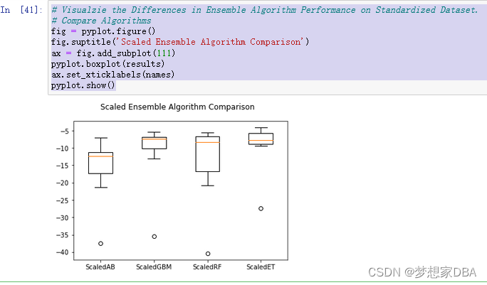
We can probably do better, given that the ensemble techniques used the default parameters. In the next section we will look at tuning the Gradient Boosting to further lift the performance.

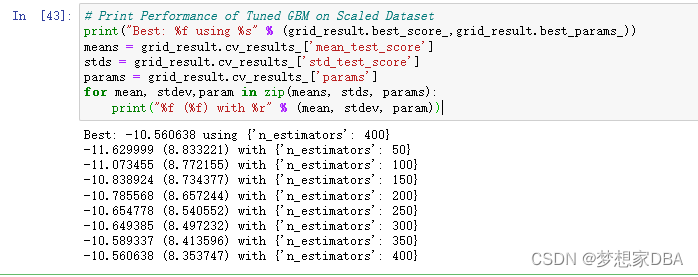
1.10 Tune Ensemble Methods

The default number of boosting stages to perform (n estimators) is 100. This is a good candidate parameter of Gradient Boosting to tune. Often, the larger the number of boosting stages, the better the performance but the longer the training time. In this section we will look at tuning the number of stages for gradient boosting. Below we define a parameter grid n estimators values from 50 to 400 in increments of 50. Each setting is evaluated using 10-fold cross validation.

# Tune scaled GBM
scaler = StandardScaler().fit(X_train)
rescaledX = scaler.transform(X_train)
param_grid = dict(n_estimators=np.array([50, 100, 150, 200, 250, 300, 350, 400]))
model = GradientBoostingRegressor(random_state=seed)
kfold = KFold(n_splits=num_folds, random_state=seed, shuffle=True)
grid = GridSearchCV(estimator=model, param_grid=param_grid, scoring=scoring, cv=kfold)
grid_result = grid.fit(rescaledX,Y_train)

As before, we can summarize the best configuration and get an idea of how performance changed with each different configuration.

# Print Performance of Tuned GBM on Scaled Dataset
print("Best: %f using %s" % (grid_result.best_score_,grid_result.best_params_))
means = grid_result.cv_results_['mean_test_score']
stds = grid_result.cv_results_['std_test_score']
params = grid_result.cv_results_['params']
for mean, stdev,param in zip(means, stds, params):
    print("%f (%f) with %r" % (mean, stdev, param))

We can see that the best configuration was n estimators=400 resulting in a mean squared error of -10.560638, about 0.65 units better than the untuned method.

11.Finalize Model

In this section, we will finalize the gradient boosting model and evaluate it on our hold out validation dataset. First we need to prepare the model and train it on the entire training dataset.This includes standardizing the training dataset before triaining.

# Construct the Finalized Model
# prepare the model
scaler = StandardScaler().fit(X_train)
rescaledX = scaler.transform(X_train)
model = GradientBoostingRegressor(random_state=seed, n_estimators=400)
model.fit(rescaledX,Y_train)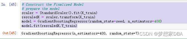

We can then scale the inputs for the validation dataset and generate predictions.

# Evaluate the Finalized Model
# transform the validation dataset
rescaledValidationX = scaler.transform(X_validation)
predictions = model.predict(rescaledValidationX)
print(mean_squared_error(Y_validation,predictions))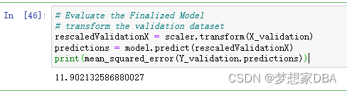

1.12 Summary

In this chapter you worked through a regression predictive modeling machine learning problem from end-to-end using Python. Specifically, the steps covered were:

Problem Definition (Boston house price data).
Loading the Dataset.
Analyze Data (some skewed distributions and correlated attributes).
Evaluate Algorithms (Linear Regression looked good).
Evaluate Algorithms with Standardization (KNN looked good).
Algorithm Tuning (K=3 for KNN was best).
Ensemble Methods (Bagging and Boosting, Gradient Boosting looked good).
Tuning Ensemble Methods (getting the most from Gradient Boosting).
Finalize Model (use all training data and confirm using validation dataset).

Working through this case study showed you how the recipes for specific machine learning tasks can be pulled together into a complete project. Working through this case study is good practice at applied machine learning using Python and scikit-learn.