MobileNet_V1 实战：手把手教你复现 MobileNet_V1

原创已于 2025-04-24 23:24:31 修改 · 1.5k 阅读

23 ·

CC 4.0 BY-SA版权

文章标签：

#深度学习 #神经网络 #分类 #目标检测

于 2025-04-24 22:58:40 首次发布

深度学习论文阅读与代码实战专栏收录该内容

2 篇文章

订阅专栏

部署运行你感兴趣的模型镜像

《MobileNet_V1 实战：手把手教你复现 MobileNet_V1》

论文地址：MobileNets: Efficient Convolutional Neural Networks for Mobile Vision Applications

文章目录

《MobileNet_V1 实战：手把手教你复现 MobileNet_V1》

1.开篇引言：

MobileNet 作为一个里程碑式的轻量级 CNN 网络，完美平衡了模型性能和计算效率。本文将带领大家从零开始，
通过 PyTorch 实现 MobileNet_V1，深入理解其架构设计和核心思想。

2.网络创新点概述：

核心创新：深度可分离卷积取代标准卷积
优势：大幅降低参数量和计算量
可调节性：通过 width multiplier 控制模型大小

3.深度可分离卷积详解：

深度可分离卷积由深度卷积（Depthwise convolutions）和逐点卷积（Pointwise convolutions）组成，我们复习一下相关的卷积：

我们这里假设输入特征图的宽度和高度为 $D_F$ ，输入通道数为 M ，输出特征图的宽度和高度为 $D_G$ ，输出通道数为 N 。卷积核的大小为 $D_K$

卷积名称	参数量	计算量
标准卷积（Standard convolution）	$D_K \times D_K \times M \times N$	$D_K \times D_K \times M \times N \times D_G \times D_G$
逐点卷积（Pointwise convolutions）	$\times 1 \times M \times N$	$\times 1 \times M \times N \times D_G \times D_G$
深度卷积（Depthwise convolutions）	$D_K \times D_K \times M$	$D_K \times D_K \times M \times D_G \times D_G$
深度可分离卷积（Depthwise separable convolution）	$D_K \times D_K \times M + M \times N$	$(D_K \times D_K \times M + M \times N)\times D_G \times D_G$

这里我们详细讲解一下参数量和计算量是如何得出的，顺便复习一下卷积知识：

（1）标准卷积（Standard Convolution）

假设：

输入特征图大小为 9×9×6（宽 × 高 × 通道数）。
卷积核大小为 3×3。
输出特征图大小为 7×7×3（宽 × 高 × 通道数）。
卷积核的步幅为 1，填充为 0。

参数量计算：

每个卷积核的大小为 3×3。
输入通道数为 6，因此每个卷积核需要 6 个通道的权重。
输出通道数为 3，因此需要 3 个卷积核组。
参数量 = 卷积核宽度 × 卷积核高度 × 输入通道数 × 输出通道数
参数量 = 3 × 3 × 6 × 3 = 162

计算量计算：

每个卷积核需要对输入特征图的每个位置进行卷积操作。
输出特征图的大小为 7×7，即每个卷积核需要计算 7×7 个位置。
每次卷积操作需要计算 3×3×6 次乘法。
总计算量 = 卷积核宽度 × 卷积核高度 × 输入通道数 × 输出通道数 × 输出特征图宽度 × 输出特征图高度
计算量 = 3 × 3 × 6 × 3 × 7 × 7 = 2,646

代码实现：

import torch
import torch.nn as nn
from torchsummary import summary

# 定义标准卷积
class StandardConv(nn.Module):
    def __init__(self):
        super(StandardConv, self).__init__()
        self.conv = nn.Conv2d(
            in_channels=6,  # 输入通道数
            out_channels=3,  # 输出通道数
            kernel_size=3,  # 卷积核大小
            stride=1,  # 步幅
            padding=0  # 填充
        )

    def forward(self, x):
        return self.conv(x)

# 输入特征图大小为 (6, 9, 9)
device = torch.device('cuda' if torch.cuda.is_available() else 'cpu')
model = StandardConv().to(device)
print(summary(model, input_size=(6, 9, 9)))

----------------------------------------------------------------
        Layer (type)               Output Shape         Param #
================================================================
            Conv2d-1              [-1, 3, 7, 7]             165
================================================================
Total params: 165
Trainable params: 165
Non-trainable params: 0
----------------------------------------------------------------
Input size (MB): 0.00
Forward/backward pass size (MB): 0.00
Params size (MB): 0.00
Estimated Total Size (MB): 0.00
----------------------------------------------------------------
None

这里我们发现参数多出了 3 个，它们是 bias，如果我们将 bias=False，那么参数就为 162，下面的参数量计算同理。

（2）深度卷积（Depthwise Convolution）

假设：

输入特征图大小为 9×9×6。
卷积核大小为 3×3。
输出特征图大小为 7×7×6（深度卷积不会改变通道数）。
卷积核的步幅为 1，填充为 0。

参数量计算

每个输入通道对应一个独立的卷积核。
每个卷积核的大小为 3×3。
输入通道数为 6，因此需要 6 个卷积核。
参数量 = 卷积核宽度 × 卷积核高度 × 输入通道数
参数量 = 3 × 3 × 6 = 54

计算量计算

每个卷积核需要对输入特征图的每个位置进行卷积操作。
输出特征图的大小为 7×7，即每个卷积核需要计算 7×7 个位置。
每次卷积操作需要计算 3×3 次乘法。
总计算量 = 卷积核宽度 × 卷积核高度 × 输入通道数 × 输出特征图宽度 × 输出特征图高度
计算量 = 3 × 3 × 6 × 7 × 7 = 882

代码实现：

class DepthwiseConv(nn.Module):
    def __init__(self):
        super(DepthwiseConv, self).__init__()
        self.conv = nn.Conv2d(
            in_channels=6,  # 输入通道数
            out_channels=6,  # 输出通道数（与输入通道数相同）
            kernel_size=3,  # 卷积核大小
            stride=1,  # 步幅
            padding=0,  # 填充
            groups=6  # 分组数等于输入通道数
        )

    def forward(self, x):
        return self.conv(x)

# 输入特征图大小为 (6, 9, 9)
model = DepthwiseConv().to(device)
print(summary(model, input_size=(6, 9, 9)))

----------------------------------------------------------------
        Layer (type)               Output Shape         Param #
================================================================
            Conv2d-1              [-1, 6, 7, 7]              60
================================================================
Total params: 60
Trainable params: 60
Non-trainable params: 0
----------------------------------------------------------------
Input size (MB): 0.00
Forward/backward pass size (MB): 0.00
Params size (MB): 0.00
Estimated Total Size (MB): 0.00
----------------------------------------------------------------
None

（3）逐点卷积（Pointwise Convolution）

假设：

输入特征图大小为 7×7×6。
卷积核大小为 1×1。
输出特征图大小为 7×7×3。
卷积核的步幅为 1，填充为 0。

参数量计算

每个卷积核的大小为 1×1。
输入通道数为 6。
输出通道数为 3。
参数量 = 卷积核宽度 × 卷积核高度 × 输入通道数 × 输出通道数
参数量 = 1 × 1 × 6 × 3 = 18

计算量计算

每个卷积核需要对输入特征图的每个位置进行卷积操作。
输出特征图的大小为 7×7，即每个卷积核需要计算 7×7 个位置。
每次卷积操作需要计算 1×1×6 次乘法。
总计算量 = 卷积核宽度 × 卷积核高度 × 输入通道数 × 输出通道数 × 输出特征图宽度 × 输出特征图高度
计算量 = 1 × 1 × 6 × 3 × 7 × 7 = 882

代码实现：

class PointwiseConv(nn.Module):
    def __init__(self):
        super(PointwiseConv, self).__init__()
        self.conv = nn.Conv2d(
            in_channels=6,  # 输入通道数
            out_channels=3,  # 输出通道数
            kernel_size=1,  # 卷积核大小
            stride=1,  # 步幅
            padding=0  # 填充
        )

    def forward(self, x):
        return self.conv(x)

# 输入特征图大小为 (6, 7, 7)
model = PointwiseConv().to(device)
print(summary(model, input_size=(6, 7, 7)))

----------------------------------------------------------------
        Layer (type)               Output Shape         Param #
================================================================
            Conv2d-1              [-1, 3, 7, 7]              21
================================================================
Total params: 21
Trainable params: 21
Non-trainable params: 0
----------------------------------------------------------------
Input size (MB): 0.00
Forward/backward pass size (MB): 0.00
Params size (MB): 0.00
Estimated Total Size (MB): 0.00
----------------------------------------------------------------
None

4.网络结构实现：

模块	操作类型	输入通道	输出通道	卷积核 / 操作	下采样（stride）
Stem	普通卷积 + 深度可分离卷积	3	64α	3×3, 3×3	1, 1
Block1	深度可分离卷积 ×2	64α	128α	3×3（两次）	2, 1
Block2	深度可分离卷积 ×2	128α	256α	3×3（两次）	2, 1
Block3	深度可分离卷积 ×6	256α	512α	3×3（六次）	2, 1, 1, 1, 1, 1
Block4	深度可分离卷积 ×2	512α	1024α	3×3（两次）	2, 1
AvgPool（平均池化）	自适应平均池化	1024α	1024α	全局池化	-
FC	全连接	1024α	class_num 类别编号	-	-

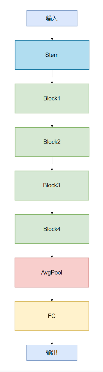
我这里仅引入宽度系数 $\alpha$ 没有使用分辨率系数 $\beta $

mobilenet.py:

""" mobilenet in pytorch
	Author：Hao | 2025/04/16
    MobileNets: Efficient Convolutional Neural Networks for Mobile Vision Applications
    https://arxiv.org/abs/1704.04861
"""

import torch
import torch.nn as nn
from torchinfo import summary


class DepthSeperabelConv2d(nn.Module):

    def __init__(self, input_channels, output_channels, kernel_size, **kwargs):
        super().__init__()
        self.depthwise = nn.Sequential(
            nn.Conv2d(
                input_channels,
                input_channels,
                kernel_size,
                groups=input_channels,
                **kwargs),
            nn.BatchNorm2d(input_channels),
            nn.ReLU(inplace=True)
        )

        self.pointwise = nn.Sequential(
            nn.Conv2d(input_channels, output_channels, 1),
            nn.BatchNorm2d(output_channels),
            nn.ReLU(inplace=True)
        )

    def forward(self, x):
        x = self.depthwise(x)
        x = self.pointwise(x)

        return x


class BasicConv2d(nn.Module):

    def __init__(self, input_channels, output_channels, kernel_size, **kwargs):

        super().__init__()
        self.conv = nn.Conv2d(
            input_channels, output_channels, kernel_size, **kwargs)
        self.bn = nn.BatchNorm2d(output_channels)
        self.relu = nn.ReLU(inplace=True)

    def forward(self, x):
        x = self.conv(x)
        x = self.bn(x)
        x = self.relu(x)

        return x


class MobileNet(nn.Module):

    """
    Args:
        width multipler: The role of the width multiplier α is to thin
                         a network uniformly at each layer. For a given
                         layer and width multiplier α, the number of
                         input channels M becomes αM and the number of
                         output channels N becomes αN.
    """

    def __init__(self, width_multiplier=1, class_num=100):
       super().__init__()

       alpha = width_multiplier
       self.stem = nn.Sequential(
           BasicConv2d(3, int(32 * alpha), 3, padding=1, bias=False),
           DepthSeperabelConv2d(
               int(32 * alpha),
               int(64 * alpha),
               3,
               padding=1,
               bias=False
           )
       )

       #downsample
       self.conv1 = nn.Sequential(
           DepthSeperabelConv2d(
               int(64 * alpha),
               int(128 * alpha),
               3,
               stride=2,
               padding=1,
               bias=False
           ),
           DepthSeperabelConv2d(
               int(128 * alpha),
               int(128 * alpha),
               3,
               padding=1,
               bias=False
           )
       )

       #downsample
       self.conv2 = nn.Sequential(
           DepthSeperabelConv2d(
               int(128 * alpha),
               int(256 * alpha),
               3,
               stride=2,
               padding=1,
               bias=False
           ),
           DepthSeperabelConv2d(
               int(256 * alpha),
               int(256 * alpha),
               3,
               padding=1,
               bias=False
           )
       )

       #downsample
       self.conv3 = nn.Sequential(
           DepthSeperabelConv2d(
               int(256 * alpha),
               int(512 * alpha),
               3,
               stride=2,
               padding=1,
               bias=False
           ),

           DepthSeperabelConv2d(
               int(512 * alpha),
               int(512 * alpha),
               3,
               padding=1,
               bias=False
           ),
           DepthSeperabelConv2d(
               int(512 * alpha),
               int(512 * alpha),
               3,
               padding=1,
               bias=False
           ),
           DepthSeperabelConv2d(
               int(512 * alpha),
               int(512 * alpha),
               3,
               padding=1,
               bias=False
           ),
           DepthSeperabelConv2d(
               int(512 * alpha),
               int(512 * alpha),
               3,
               padding=1,
               bias=False
           ),
           DepthSeperabelConv2d(
               int(512 * alpha),
               int(512 * alpha),
               3,
               padding=1,
               bias=False
           )
       )

       #downsample
       self.conv4 = nn.Sequential(
           DepthSeperabelConv2d(
               int(512 * alpha),
               int(1024 * alpha),
               3,
               stride=2,
               padding=1,
               bias=False
           ),
           DepthSeperabelConv2d(
               int(1024 * alpha),
               int(1024 * alpha),
               3,
               padding=1,
               bias=False
           )
       )

       self.fc = nn.Linear(int(1024 * alpha), class_num)
       self.avg = nn.AdaptiveAvgPool2d(1)

    def forward(self, x):
        x = self.stem(x)

        x = self.conv1(x)
        x = self.conv2(x)
        x = self.conv3(x)
        x = self.conv4(x)

        x = self.avg(x)
        x = x.view(x.size(0), -1)
        x = self.fc(x)
        return x


def mobilenet(alpha=1, class_num=10):
    return MobileNet(alpha, class_num)

# 测试代码
if __name__ == "__main__":
    model = mobilenet(class_num=10)  # 10 分类任务
    x = torch.randn(1, 3, 224, 224)  # 输入张量
    y = model(x)  # 前向传播
    print("输出形状:", y.shape)  # 输出形状
    summary(model, input_size=(1, 3, 224, 224))  # 打印模型摘要

5.CIFAR-10实战

train.py:

import torch
import torch.nn as nn
import torch.optim as optim
import torchvision
import torchvision.transforms as transforms
from mobilenet import mobilenet
from torch.utils.data import DataLoader
import matplotlib.pyplot as plt

# 设置设备
device = torch.device("cuda" if torch.cuda.is_available() else "cpu")

# 数据预处理
transform_train = transforms.Compose([
    transforms.RandomCrop(32, padding=4),
    transforms.RandomHorizontalFlip(),
    transforms.ToTensor(),
    transforms.Normalize((0.4914, 0.4822, 0.4465), (0.2023, 0.1994, 0.2010)),
])

transform_test = transforms.Compose([
    transforms.ToTensor(),
    transforms.Normalize((0.4914, 0.4822, 0.4465), (0.2023, 0.1994, 0.2010)),
])

# 加载CIFAR10数据集
trainset = torchvision.datasets.CIFAR10(
    root='./data', train=True, download=False, transform=transform_train)
trainloader = DataLoader(trainset, batch_size=128, shuffle=True, num_workers=2)

testset = torchvision.datasets.CIFAR10(
    root='./data', train=False, download=False, transform=transform_test)
testloader = DataLoader(testset, batch_size=100, shuffle=False, num_workers=2)

# 类别标签
classes = ('plane', 'car', 'bird', 'cat', 'deer',
           'dog', 'frog', 'horse', 'ship', 'truck')

# 创建模型
model = mobilenet(alpha=1, class_num=10).to(device)

# 定义损失函数和优化器
criterion = nn.CrossEntropyLoss()
optimizer = optim.SGD(model.parameters(), lr=0.1, momentum=0.9, weight_decay=5e-4)
scheduler = optim.lr_scheduler.CosineAnnealingLR(optimizer, T_max=200)

# 训练函数
def train(epoch):
    model.train()
    train_loss = 0
    correct = 0
    total = 0
    
    for batch_idx, (inputs, targets) in enumerate(trainloader):
        inputs, targets = inputs.to(device), targets.to(device)
        optimizer.zero_grad()
        outputs = model(inputs)
        loss = criterion(outputs, targets)
        loss.backward()
        optimizer.step()

        train_loss += loss.item()
        _, predicted = outputs.max(1)
        total += targets.size(0)
        correct += predicted.eq(targets).sum().item()

        if batch_idx % 100 == 0:
            print(f'Epoch: {epoch}, Batch: {batch_idx}, Loss: {train_loss/(batch_idx+1):.3f}, '
                  f'Acc: {100.*correct/total:.2f}%')

# 测试函数
def test(epoch):
    model.eval()
    test_loss = 0
    correct = 0
    total = 0
    
    with torch.no_grad():
        for inputs, targets in testloader:
            inputs, targets = inputs.to(device), targets.to(device)
            outputs = model(inputs)
            loss = criterion(outputs, targets)

            test_loss += loss.item()
            _, predicted = outputs.max(1)
            total += targets.size(0)
            correct += predicted.eq(targets).sum().item()

    print(f'Epoch: {epoch}, Test Loss: {test_loss/len(testloader):.3f}, '
          f'Test Acc: {100.*correct/total:.2f}%')
    
    return 100.*correct/total


def main():
    # 训练模型
    best_acc = 0
    epochs = 20

    for epoch in range(epochs):
        train(epoch)
        acc = test(epoch)
        scheduler.step()

        # 保存最佳模型
        if acc > best_acc:
            print(f'Saving best model with accuracy: {acc}%')
            torch.save(model.state_dict(), 'mobilenet_cifar10_best.pth')
            best_acc = acc

    print(f'Best accuracy: {best_acc}%')


if __name__ == '__main__':
    # 在Windows下使用多进程时需要添加freeze_support()
    from multiprocessing import freeze_support

    freeze_support()
    main()

save_cifar10_images.py:

import torch
import torchvision
import torchvision.transforms as transforms
import matplotlib.pyplot as plt
import numpy as np
from PIL import Image
import os

def save_cifar10_images(num_images=10, save_dir='test_images'):
    """从CIFAR-10测试集中保存图片"""
    # 创建保存目录
    if not os.path.exists(save_dir):
        os.makedirs(save_dir)
    
    # 加载CIFAR-10测试集
    transform = transforms.ToTensor()
    testset = torchvision.datasets.CIFAR10(
        root='./data', train=False, download=False, transform=transform)
    
    # 类别名称
    classes = ('plane', 'car', 'bird', 'cat', 'deer',
              'dog', 'frog', 'horse', 'ship', 'truck')
    
    # 为每个类别保存图片
    for class_idx in range(10):
        # 获取该类别的所有图片索引
        class_indices = [i for i, (_, label) in enumerate(testset) if label == class_idx]
        
        # 随机选择一张该类别的图片
        if class_indices:
            img_idx = np.random.choice(class_indices)
            image, label = testset[img_idx]
            
            # 转换为PIL图像
            image = transforms.ToPILImage()(image)
            
            # 保存图片
            save_path = os.path.join(save_dir, f'{classes[label]}_{img_idx}.png')
            image.save(save_path)
            print(f'Saved {classes[label]} image to {save_path}')

def show_random_test_images(num_images=5):
    """显示并测试随机的测试集图片"""
    # 加载测试集
    transform = transforms.ToTensor()
    testset = torchvision.datasets.CIFAR10(
        root='./data', train=False, download=False, transform=transform)
    
    # 类别名称
    classes = ('plane', 'car', 'bird', 'cat', 'deer',
              'dog', 'frog', 'horse', 'ship', 'truck')
    
    # 随机选择图片索引
    indices = np.random.choice(len(testset), num_images, replace=False)
    
    # 创建子图
    fig, axes = plt.subplots(1, num_images, figsize=(15, 3))
    
    # 显示每张图片
    for i, idx in enumerate(indices):
        image, label = testset[idx]
        image = transforms.ToPILImage()(image)
        
        axes[i].imshow(image)
        axes[i].set_title(f'Class: {classes[label]}')
        axes[i].axis('off')
    
    plt.tight_layout()
    plt.show()

def main():
    # 1. 保存一些测试图片到本地
    print("Saving CIFAR-10 test images...")
    save_cifar10_images(num_images=10, save_dir='test_images')
    
    # 2. 显示一些随机的测试图片
    print("\nShowing random test images...")
    show_random_test_images(num_images=5)

if __name__ == '__main__':
    main()

test.py:

import torch
import torchvision
import torchvision.transforms as transforms
from models.mobilenet import mobilenet
from torch.utils.data import DataLoader
from PIL import Image
import matplotlib.pyplot as plt
import numpy as np
import os
print("当前工作目录:", os.getcwd())
# 设置设备
device = torch.device("cuda" if torch.cuda.is_available() else "cpu")

# 类别标签
classes = ('plane', 'car', 'bird', 'cat', 'deer',
           'dog', 'frog', 'horse', 'ship', 'truck')

def load_model():
    """加载训练好的模型"""
    model = mobilenet(alpha=1, class_num=10).to(device)
    model.load_state_dict(torch.load('./train_models/mobilenet_cifar10_best.pth'))
    model.eval()
    return model

def test_on_testset():
    """在整个测试集上评估模型"""
    # 数据预处理
    transform_test = transforms.Compose([
        transforms.ToTensor(),
        transforms.Normalize((0.4914, 0.4822, 0.4465), (0.2023, 0.1994, 0.2010)),
    ])

    # 加载测试集
    testset = torchvision.datasets.CIFAR10(
        root='./data', train=False, download=False, transform=transform_test)
    testloader = DataLoader(testset, batch_size=100, shuffle=False, num_workers=2)

    # 加载模型
    model = load_model()
    
    # 测试
    correct = 0
    total = 0
    class_correct = [0] * 10
    class_total = [0] * 10
    
    with torch.no_grad():
        for images, labels in testloader:
            images, labels = images.to(device), labels.to(device)
            outputs = model(images)
            _, predicted = torch.max(outputs.data, 1)
            total += labels.size(0)
            correct += (predicted == labels).sum().item()
            
            # 统计每个类别的准确率
            c = (predicted == labels).squeeze()
            for i in range(labels.size(0)):
                label = labels[i]
                class_correct[label] += c[i].item()
                class_total[label] += 1

    # 打印总体准确率
    print(f'Overall Accuracy on test set: {100 * correct / total:.2f}%')
    
    # 打印每个类别的准确率
    for i in range(10):
        print(f'Accuracy of {classes[i]}: {100 * class_correct[i] / class_total[i]:.2f}%')

def predict_single_image(image_path):
    """预测单张图片"""
    # 图像预处理
    transform = transforms.Compose([
        transforms.Resize((32, 32)),
        transforms.ToTensor(),
        transforms.Normalize((0.4914, 0.4822, 0.4465), (0.2023, 0.1994, 0.2010)),
    ])
    
    # 加载并处理图像
    image = Image.open(image_path)
    image_tensor = transform(image).unsqueeze(0).to(device)
    
    # 加载模型并预测
    model = load_model()
    
    with torch.no_grad():
        outputs = model(image_tensor)
        probabilities = torch.nn.functional.softmax(outputs, dim=1)
        probability, predicted = torch.max(probabilities, 1)
        
    return classes[predicted.item()], probability.item()

def visualize_prediction(image_path):
    """可视化预测结果"""
    # 加载原始图像
    image = Image.open(image_path)
    
    # 获取预测结果
    pred_class, confidence = predict_single_image(image_path)
    
    # 显示图像和预测结果
    plt.figure(figsize=(6, 6))
    plt.imshow(image)
    plt.axis('off')
    plt.title(f'Prediction: {pred_class}\nConfidence: {confidence:.2f}')
    plt.show()

def main():
    # 1. 测试整个测试集
    print("Testing on the entire test set...")
    test_on_testset()
    
    # 2. 测试单张图片
    print("\nTesting single image prediction...")
    image_path = 'path/to/your/test/image.jpg'  # 替换为你的测试图片路径
    try:
        pred_class, confidence = predict_single_image(image_path)
        print(f'Predicted class: {pred_class}')
        print(f'Confidence: {confidence:.2f}')
        
        # 可视化结果
        visualize_prediction(image_path)
    except Exception as e:
        print(f"Error processing image: {e}")

if __name__ == '__main__':
    main()

文章到这里就结束了，如果有任何问题，欢迎讨论。

您可能感兴趣的与本文相关的镜像

PyTorch 2.6

PyTorch

Cuda

PyTorch 是一个开源的 Python 机器学习库，基于 Torch 库，底层由 C++ 实现，应用于人工智能领域，如计算机视觉和自然语言处理