


 本文深入浅出地介绍了神经网络的基础概念,从单层感知器处理线性可分问题出发,详细解析了其数学模型和学习算法。同时,文章对比了Adaline神经元的原理与实现,展示了如何通过梯度下降法最小化平方误差,达到优化权重的目的。
1. 初级的神经网络
单层感知器是用来处理线性可分问题。
线性可分简单的说,如果二维平面上有两类点,然后可以用一条直线一刀切,类似可以扩展到n维。
既然只有两类,就可以用01函数(hardlim)来作为刀,这里叫输出函数,也叫阈值函数。
输入呢有n多,怎么办?sigma(和)一下,就只有一个了。
老是和的话就总是一样的数值了,怎么办?那就加权吧,就是对每个x[i]都有一个特定权值w[i],然后相乘再相加。
最后弄个偏移量b,多加一个x[0]=1,b=w[0],这个小技巧就很方便编程了。
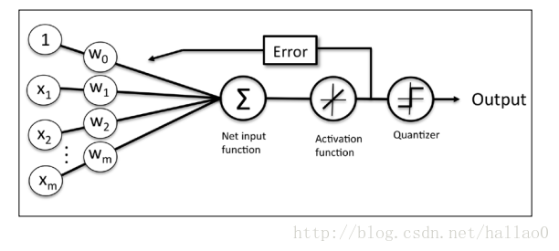
模型如下:模型
数学表示:y=hardlim(sigma(w[i]*x[i])) , i=0-n
判决平面:
sigma(w[i]*x[i])=0;
学习算法:
(1) 设置变量和参数:
X(n)= [1,x1 (n),x2 (n),…,xm (n)]为输入向量;
W(n)= [b (n),w1 (n),w2 (n),…,wm (n)]为权值向量;
b (n)为偏差; y (n)为感知器实际输出;
d (n)为期望输出; n为迭代次数;
η为学习速率,对于单层感知器 ,设η =1.
(2) 初始化 n=0,权值向量Wj(0)=[各一个较小的随机非零数]
(3) 对于一组输入样本X(n),指定它的期望输出y(0|1)
(4) 计算感知器实际输出 d=hardlim(sigma), e=y[i]-d;
(5) 调整感知器的权值向量 w[i]new=w[i]old+x[i]*e;
(6)满足条件?是,结束; 否,n增加1,转第三步。
注意:判断满足条件可以是:
(1) 误差小,即|d(n)-y(n)|<ε ;
(2) 权值变化小,即|w(n+1)-w(n)|<ε ;
(3) 超过设定的最大迭代次数。
#include <stdio.h>
#include <time.h>
#include <math.h>
#include <stdlib.h>

#define M 4  //样本数
#define N 3  //样本维度
#define Max 10 // 最大次数
#define eps 1e-4

inline int hardlim(double a){ return (a>eps)?1:0; }

double x[M][N]={
		{1, 0, 0},
		{1, 0, 1},
		{1, 1, 0},
		{1, 1, 1}
};
double y[M]={0,1,1,1};
double w[N];

void begin()
{
	int i, j;
	printf("title: =====ANN==adaline==与门实现=====\n");
	printf("\nbegin: \n");
	printf("	x[0]		x[1]		x[2]		y\n");
	for(i=0; i<M; ++i){
		for(j=0; j<N; ++j){		printf("	%lf", x[i][j]);		}
        printf("	%lf\n", y[i]);
	}
}

void train()
{
	int i, j, ok, tim, v;
	double e, d, sigma;

	printf("\n\ntrain: \n");
	srand(time(0));
	for(i=0; i<N; ++i){	w[i]=rand()/(RAND_MAX+1.0);	}
	printf("	e[0]		e[1]		e[2]		e[4]		ok\n");
	tim=0; v=1; // 学习速率
	while(1){
		ok=1;
		for(i=0; i<M; ++i){
			sigma=0;
			for(j=0; j<N; ++j){	sigma+=x[i][j]*w[j];		}
			d=hardlim(sigma);
			e=y[i]-d;

			printf("	%lf ", e);
			if(fabs(e)>eps) ok=0;      //fabs:求绝对值

			for(j=0; j<N; ++j){		w[j]+=v*e*x[i][j];		}
		}
		tim++;
		puts(ok?"	Y":"	N");
		if(ok || tim>Max) break;
	}
}

void test(){
	int i, j;
	double sigma;

	printf("\n\ntest: \n");
	printf("	x[0]		x[1]		x[2]		sigma		ans\n");
	for(i=0; i<M; ++i){
		sigma=0;
		for(j=0; j<N; ++j){
			printf("	%lf", x[i][j]);
			sigma+=x[i][j]*w[j];
		}
		printf("	%lf	", sigma);
		printf("%d\n", hardlim(sigma));
	}
	puts("==end==");
}

int main()
{
	begin();
	train();
	test();
	return 0;
}
运行结果:
title: =====ANN==adaline==与门实现=====

begin:
        x[0]            x[1]            x[2]            y
        1.000000        0.000000        0.000000        0.000000
        1.000000        0.000000        1.000000        0.000000
        1.000000        1.000000        0.000000        0.000000
        1.000000        1.000000        1.000000        1.000000


train:
        e[0]            e[1]            e[2]            e[4]            ok
        -1.000000       0.000000        0.000000        0.000000        N
        0.000000        0.000000        0.000000        0.000000        Y


test:
        x[0]            x[1]            x[2]            sigma           ans
        1.000000        0.000000        0.000000        -0.434174       0
        1.000000        0.000000        1.000000        -0.284882       0
        1.000000        1.000000        0.000000        -0.069977       0
        1.000000        1.000000        1.000000        0.079315        1
==end==
Press any key to continue
2. Adaline
2.1 Adaline原理
一个初级的一层神经网,这是在最初级上面的follow up 版。
增强的点有:
1. Bernard新提出了cost function
2. weights的更新基于线性方程(linear activation function),而不是之前perceptron中的离散方程(unit step function)
Cost Function
Sum of Square Errors(SSE) 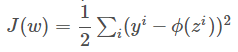
其中![]() 为图中Activation function的输出,在此处简单定义为:
为图中Activation function的输出,在此处简单定义为: ![]()
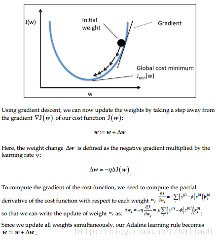
理想的状况是,目标方程是U型的。我们可以用梯度下降法找到最小的cost.
梯度下降gradient descent
η为步长, 偏导结果为方向
feature scaling
当η过大时,会发生overshoot. 解决办法一个是减小它的大小,另外一种办法是特征缩放。在此次实验中用的是标准化的方法缩小特征值。
2.2 实现
import numpy as np
class AdalineGD(object):
    """ADAptive LInear NEuron classifier.
    Parameters
    -----------
    eta : float
    Learning rate (between 0.0 and 1.0)
    n_iter : int
    Passes over the training dataset.

    Attributes
    -----------
    w_ : 1d-array
    Weights after fitting.
    errors_ : list
    Number of misclassifications in every epoch.
    """
    def __init__(self, eta=0.01, n_iter=50):
        self.eta = eta
        self.n_iter = n_iter
    def fit(self, X, y):
    """ Fit training data.

    Parameters
    ----------
    X : {array-like}, shape = [n_samples, n_features]
        Training vectors, where n_samples is the number of samples and
        n_features is the number of features.
    y : array-like, shape = [n_samples]Target values.

    Returns
    -------
    self : object
    """
        self.w_ = np.zeros(1 + X.shape[1])
        self.cost_ = []
        for i in range(self.n_iter):
            output = self.net_input(X)
            errors = (y - output)
            #X.T.dot 叉乘 output:向量
            self.w_[1:] += self.eta * X.T.dot(errors)
            self.w_[0] += self.eta * errors.sum()
            cost = (errors**2).sum() / 2.0
            self.cost_.append(cost)
        return self
    def net_input(self, X):
    """Calculate net input"""
        #np.dot 点乘 output:标量
        return np.dot(X, self.w_[1:]) + self.w_[0]
    def activation(self, X):
    """Compute linear activation"""
        return self.net_input(X)
    def predict(self, X):
    """Return class label after unit step"""
        return np.where(self.activation(X) >= 0.0, 1, -1)
重点是weight的更新:
self.w_[1:] += self.eta * X.T.dot(errors)
self.w_[0] += self.eta * errors.sum()
新添的activation function:
def activation(self, X):
    """Compute linear activation"""
    return self.net_input(X)
测试
>>> fig, ax = plt.subplots(nrows=1, ncols=2, figsize=(8, 4))
>>> ada1 = AdalineGD(eta=0.01, n_iter=50).fit(X, y)
>>> ax[0].plot(range(1, len(ada1.cost_) + 1),
... np.log10(ada1.cost_), marker='o')
>>> ax[0].set_xlabel('Epochs')
>>> ax[0].set_ylabel('log(Sum-squared-error)')
>>> ax[0].set_title('Adaline - Learning rate 0.01')
>>> ada2 = AdalineGD(eta=0.0001, n_iter=50).fit(X, y)
>>> ax[1].plot(range(1, len(ada2.cost_) + 1),
... ada2.cost_, marker='o')
>>> ax[1].set_xlabel('Epochs')
>>> ax[1].set_ylabel('Sum-squared-error')
>>> ax[1].set_title('Adaline - Learning rate 0.0001')
>>> plt.show()
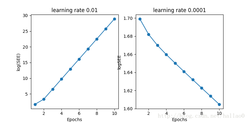
左图中,因为learning rate步长太大,发生了overshoot,所以最后没有降下来。
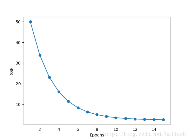
通过feature scaling, 在此也就是标准化特征:
#减去平均数,除以标准差
>>> X_std = np.copy(X)
>>> X_std[:,0] = (X[:,0] - X[:,0].mean()) / X[:,0].std()
>>> X_std[:,1] = (X[:,1] - X[:,1].mean()) / X[:,1].std()
再将模型fit函数输入改为x_std:
ada.fit(X_std, y)


 960
960

 被折叠的 条评论
为什么被折叠?
被折叠的 条评论
为什么被折叠?
 到【灌水乐园】发言


