数模MATLAB第一课_多项式拟合等

最新推荐文章于 2022-07-21 14:06:23 发布

shatterer

最新推荐文章于 2022-07-21 14:06:23 发布

阅读量725

点赞数 1

CC 4.0 BY-SA版权

分类专栏： MATLAB 文章标签： MATLAB

本文链接：https://blog.youkuaiyun.com/shatterer/article/details/79884923

MATLAB 专栏收录该内容

1 篇文章

订阅专栏

本文介绍了MATLAB中进行二维线图绘制和多项式拟合的方法，包括plot函数的使用，polyfit指令拟合多项式，以及曲线拟合工具箱的基本操作。详细讲解了polyfit函数的使用和图形窗口的拟合过程，并提到了非线性函数的拟合示例。

摘要生成于 C知道，由 DeepSeek-R1 满血版支持，前往体验 >

MATLAB预备知识：

二维线图：plot

plot（x）；plot（x， y）； plot（x, y, LineSpec) ;

常用颜色有红'r'、绿 'g'、蓝 'b'、品红'm'、黑'k' 等

线型有点画线'.-'、虚线'-'、点连线'.'、

点型有星形符'*'、圆形'o'、加号'+'等更多。颜色和线形可以分别也可以组合使用,如下就是点型、线型、颜色同时使用。

>> x = [1 2 3 4 5 6 7 8 9];
>> y = [9 7 6 3 -1 2 5 7 20];
>> plot(x, 'b*');
>> hold on % 使用此函数可以继续在画布上作图
>> plot(x, y, 'r:.')
>> hold off % 停止在画布上作图

1.2.1多项式拟合

指令语句拟合

polyfit（）多项式拟合(在最小二乘方式中），返回拟合的系数。
如p = polyfit(x, y, n)% 返回阶数为n的多项式系数，f1 里应有n + 1 个数
[p, S] = polyfit（）以及[p, S, mu]输出详见文档
polyval（f1, x）将计算以f1为多项式系数的函数在x点处的值。

图形窗口的多项式拟合

先用plot（）绘出y的数据，然后点击tool→basic fit。

1.2.2指定多项式拟合

使用fittype函数
fittype（'函数体'，'independent','x', 'coefficients', {'a', 'k', 'w'})
还可以添加的其他参数见文档

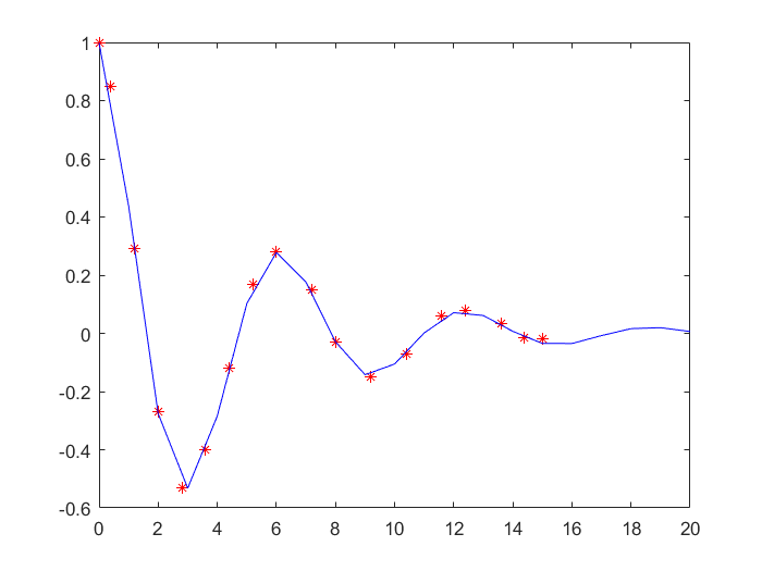
1.使用非线性函数‘a*cos（kt）*exp（w*t）’来拟合数据：

syms t;
x = [0 0.4 1.2 2 2.8 3.6 4.4 5.2 6 7.2 8 9.2 10.4 11.6 12.4 13.6 14.4 15]'; % 后面加个 单引号，表转置
y = [1 0.85 0.29 -0.27 -0.53 -0.4 -0.12 0.17 0.28 0.15 -0.03 -0.15 -0.071 0.059 0.08 0.032 -0.015 -0.02]';
f = fittype('a * cos(k * t) * exp(w * t)', 'coefficients', {'a', 'k', 'w'}, 'independent', 't'); % coefficients是参数， independent自变量，dependent因变量
cfun = fit(x, y, f); % fit函数的参数必须是列向量（暂时不知道是为什么）
xi = 0 : 1: 20;
yi = cfun(xi);
plot(x, y, 'r*', xi, yi, 'b-');

结果如图所示。

2.fittype()用于线形模型也很简单

用形式如 a * x + b * cos(x) + c来拟合：

<<fit1 = fittype({'x', 'cos(x)', '1'}, 'coefficients', {'a1', 'a2', 'a3'}) % coefficicents作用是给参数命名，可以不加。

fit1 =
Linear model:

fit1(a1,a2,a3,x) = a1*x + a2*cos(x) + a3

1.2.3 曲线拟合工具箱（Curve fitting tool）

功能强大，使用方便，第一次matlab作业全靠它。呼出方法很多，

在matlab2017a 中，工具栏中APP第一个工具就是curve fitting tool。点击就开。
命令栏直接输入 cftool 回车也能打开。

使用方法：目前只会用custom equation （自定义等式）来拟合，拟合结果在Results 框框查看。