


Part Ⅲ
3.1 Words list
- over fitting 过拟合
- under fitting 欠拟合
- locally weighted linear regression 局部加权线性回归
- parametric learning algorithm 参数学习算法
- exponential decay function 指数衰减函数
- maximum likelihood 似然最大化
- digression 插话
- perception learning algorithm 感知器学习算法
3.2 over fitting and under fitting
The over fitting is which make the hypothesis become over strict for getting the consistent hypothesis. And the under fitting is which has the same bad performance in training sets and test sets,it’s also be known as a bad generalization.
3.3 locally weighted regression
In the original linear regression algorithm , to make a prediction at query point xxx (i.e.,toevaluateh(x))(i.e.,to evaluate h(x))(i.e.,toevaluateh(x)), we would:
1.Fit θ\thetaθ to minimize ∑i(y(i)−θTx(i))2\sum_i(y^{(i)} - \theta^Tx^{(i)})^2∑i(y(i)−θTx(i))2.
2.Output θTx\theta^TxθTx.
In contrast, the locally weighted linear regression algorithm does the following:
1.Fit θ\thetaθ to minimize ∑iw(i)(y(i)−θTx(i))2\sum_iw(i)(y^{(i)} - \theta^Tx^{(i)})^2∑iw(i)(y(i)−θTx(i))2.
2.Output θT\theta^TθT.
Here,the w(i)w(i)w(i)'s are non_negative valued weights.Note that the weights depend on the particular point xxx at which we’re trying to evaluate xxx.In other word, the xxx is decided of you.The closer the observed points x(i)x^{(i)}x(i) is to x,the w(i)w(i)w(i) is bigger.
The fairly standard choice for the weights is:
w(i)=−exp(x(i)−x)22τ2w(i) = \frac{-exp(x^{(i)} - x)^2}{2\tau^2}w(i)=2τ2−exp(x(i)−x)2.
τ\tauτ is called the bandwidth parameter, the larger τ\tauτ is,the faster the point farther from the distance x falls.Locally weighted linear regression is the first example we’re seeing of a non-parametric algorithm.
The difference between parametric algorithm and non-parametric algorithm:
The (unweighted) linear regression algorithm that we saw earlier is known as a parametric learning algorithm, because it has a fixed, finite number of parameters (the θi’s), which are fit to the data. Once we’ve fit the θi’s and stored them away, we no longer need to keep the training data around to make future predictions. In contrast, to make predictions using locally weighted linear regression, we need to keep the entire training set around. The term “non-parametric” (roughly) refers to the fact that the amount of stuff we need to keep in order to represent the hypothesis h grows linearly with the size of the training set.
3.4 Classification logistic regression
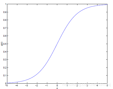
hθ(x)=g(θTx)=11+e−θTxh_\theta(x) = g(\theta^Tx) = \frac{1}{1+e^{-\theta^Tx}}hθ(x)=g(θTx)=1+e−θTx1,where g(z)=11+e−zg(z) = \frac{1}{1+e^{-z}}g(z)=1+e−z1
is called the logistic function or sigmoid function. Here is a plot showing g(z)g(z)g(z).
The derivative of the sigmoid function g′(z)=g(z)(1−g(z))g^{'}(z) = g(z)(1 - g(z))g′(z)=g(z)(1−g(z)).
Let us assume that
P(y=1∣x;θ)=hθ(x)P(y=1|x;\theta) = h_\theta(x)P(y=1∣x;θ)=hθ(x).
P(y=0∣x;θ)=1−hθ(x)P(y=0|x;\theta) = 1 - h_\theta(x)P(y=0∣x;θ)=1−hθ(x).
Note that this can be written more compactly as
P(hθ(x))y(1−hθ(x))1−yP(h_\theta(x))^y(1 - h_\theta(x))^{1-y}P(hθ(x))y(1−hθ(x))1−y.
We can solve parameters of this model by maximize the log likelihood,so we get
θj:=θj+α(y(i)−hθ(x(i)))xj(i)\theta_j:=\theta_j+\alpha(y^{(i)} - h_\theta(x^{(i)}))x^{(i)}_jθj:=θj+α(y(i)−hθ(x(i)))xj(i).
As AndrewNgAndrew NgAndrewNg side,“If we compare this to the LMSLMSLMS update rule, we see that it looks identical; but this is not the same algorithm, because hθ(x(i))h_\theta(x^{(i)})hθ(x(i)) is now defined as a non-linear function of θTx(i)θ^Tx(i)θTx(i). Nonetheless, it’s a little surprising that we end up with the same update rule for a rather different algorithm and learning problem. Is this coincidence, or is there a deeper reason behind this? We’ll answer this when get get to GLMGLMGLM models.”
3.4 The perception learning algorithm
g is a threshold function be defined:
g(x)={1ifz≥00ifz<0g(x) = \begin{cases} 1\quad if \quad z \geq0 \\ 0\quad if \quad z<0\end{cases}g(x)={1ifz≥00ifz<0.
let hθ(x)=g(θTx)h_\theta(x) = g(\theta^Tx)hθ(x)=g(θTx) and we use the update rule:
θj:=θj+α(y(i)−hθ(x(i)))xj(i)\theta_j:=\theta_j+\alpha(y^{(i)} - h_\theta(x^{(i)}))x^{(i)}_jθj:=θj+α(y(i)−hθ(x(i)))xj(i).
then we have the perception learning algorithm.


 743
743

 被折叠的 条评论
为什么被折叠?
被折叠的 条评论
为什么被折叠?
 到【灌水乐园】发言


