 RNN Encoder-Decoder在机器翻译中的应用及GRU解析


 本文是《Learning Phrase Representations using RNN Encoder–Decoder for Statistical Machine Translation》论文的学习笔记,介绍了RNN Encoder-Decoder模型在机器翻译中的应用,包括GRU结构,并探讨了其与传统SMT系统的结合。通过实验展示了模型在WMT'14 En-Fr任务上的效果。
论文: L e a r n i n g Learning Learning P h r a s e Phrase Phrase R e p r e s e n t a t i o n s Representations Representations u s i n g using using R N N RNN RNN E n c o d e r − D e c o d e r Encoder-Decoder Encoder−Decoder f o r for for S t a t i s t i c a l Statistical Statistical M a c h i n e Machine Machine T r a n s l a t i o n Translation Translation学习笔记
前言
我们知道, S e q 2 S e q Seq2Seq Seq2Seq 现在已经成为了机器翻译、对话聊天、文本摘要等工作的重要模型,真正提出 S e q 2 S e q Seq2Seq Seq2Seq 的文章是 《 S e q u e n c e 《Sequence 《Sequence t o to to S e q u e n c e Sequence Sequence L e a r n i n g Learning Learning w i t h with with N e u r a l Neural Neural N e t w o r k s 》 Networks》 Networks》,但本篇 《 L e a r n i n g 《Learning 《Learning P h r a s e Phrase Phrase R e p r e s e n t a t i o n s Representations Representations u s i n g using using R N N RNN RNN E n c o d e r – D e c o d e r Encoder–Decoder Encoder–Decoder f o r for for S t a t i s t i c a l Statistical Statistical M a c h i n e Machine Machine T r a n s l a t i o n 》 Translation》 Translation》比前者更早使用了 S e q 2 S e q Seq2Seq Seq2Seq 模型来解决机器翻译的问题,本文是该篇论文的概述。
论文地址:Learning Phrase Representations using RNN Encoder–Decoder for Statistical Machine Translation
2014 2014 2014 年 6 6 6 月发布于 A r x i v Arxiv Arxiv 上,一作是 K y u n g h y u n Kyunghyun Kyunghyun C h o Cho Cho,当时来自蒙特利尔大学,现在在纽约大学任教。
目录
- 摘要
- R N N RNN RNN
-
R
N
N
E
n
c
o
d
e
r
−
D
e
c
o
d
e
r
RNN Encoder-Decoder
RNNEncoder−Decoder
- E n c o d e r Encoder Encoder
- D e c o d e r Decoder Decoder
- E n c o d e r + D e c o d e r Encoder+Decoder Encoder+Decoder
- 新的隐藏单元
- S M T SMT SMT模型和 R N N RNN RNN E n c o d e r − D e c o d e r Encoder-Decoder Encoder−Decoder的结合
- 实验
- 代码实现
摘要
这篇论文中提出了一种新的模型,叫做 R N N RNN RNN E n c o d e r − D e c o d e r , Encoder-Decoder, Encoder−Decoder, 并将它用来进行机器翻译和比较不同语言的短语/词组之间的语义近似程度。这个模型由两个 R N N RNN RNN 组成,其中 E n c o d e r Encoder Encoder 用来将输入的序列表示成一个固定长度的向量, D e c o d e r Decoder Decoder 则使用这个向量重建出目标序列,这两个 R N N RNN RNN共同被训练,以最大化输出目标序列的概率。另外该论文提出了 G R U GRU GRU 的基本结构,为后来的研究奠定了基础。
因此本文的主要贡献是:
- 提出了一种类似于 L S T M LSTM LSTM 的 G R U GRU GRU 结构,并且具有比 L S T M LSTM LSTM 更少的参数,更不容易过拟合。
- 较早地将 S e q 2 S e q Seq2Seq Seq2Seq 应用在了机器翻译领域,并且取得了不错的效果。
R N N RNN RNN
- 论文的在介绍模型之前介绍了一下基本的循环神经网络 ( R N N ) (RNN) (RNN)的构成,熟悉这部分的可以跳过这部分,想要了解更多关于 R N N RNN RNN的思想和细节欢迎来看我之前的博客:循环神经网络介绍及其实现
循环神经网络的结构
首先看一个简单的循环神经网络,它由输入层、一个隐藏层和一个输出层组成,如下图所示:
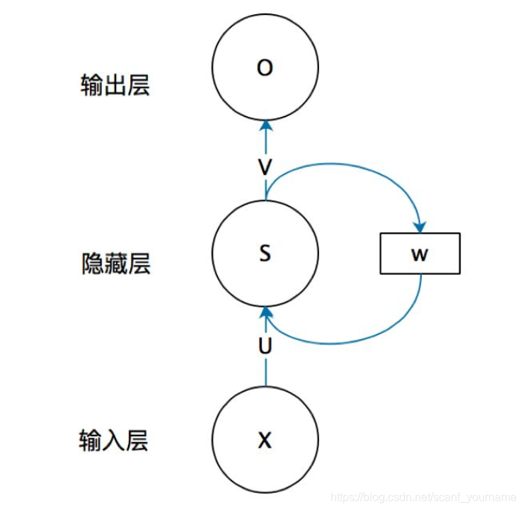
如果把上面有
W
W
W的那个带箭头的圈去掉,它就变成了最普通的全连接神经网络。
x
x
x是一个向量,它表示输入层的值(这里面没有画出来表示神经元节点的圆圈);
s
s
s是一个向量,它表示隐藏层的值(这里隐藏层面画了一个节点,你也可以想象这一层其实是多个节点,节点数与向量
s
s
s的维度相同);
U U U是输入层到隐藏层的权重矩阵, o o o也是一个向量,它表示输出层的值; V V V是隐藏层到输出层的权重矩阵。
那么,现在我们来看看 W W W是什么。循环神经网络的隐藏层的值 s s s不仅仅取决于当前这次的输入 x x x,还取决于上一次隐藏层的值 s s s。权重矩阵 W W W就是隐藏层上一次的值作为这一次的输入的权重。
我们给出这个抽象图对应的具体图:
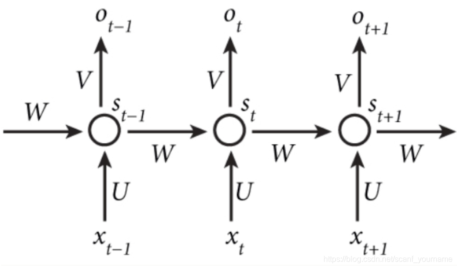
现在看上去就比较清楚了,这个网络在t时刻接收到输入
x
t
x_{t}
xt之后,隐藏层的值是
s
t
s_{t}
st ,输出值是o_{t}。关键一点是,
o
t
o_{t}
ot的值不仅仅取决于
s
t
s_{t}
st,还取决于
s
t
−
1
s_{t-1}
st−1 。我们可以用下面的公式来表示循环神经网络的计算方法:

论文中的细节
- 论文中规定模型的输入序列是 X = ( x 1 , . . . , x T ) , X=(x_{1},...,x_{T}), X=(x1,...,xT),内部的隐藏状态为 h h h(上文所述 S S S),每个时刻 t t t可以选择输出为 y t y_{t} yt,注意因为本文实现的是一个机器翻译模型,所以输入和输出可能长度不是相同的,故不一定每一个时刻都会有一个输入与之对应,一个时刻也可以对应输出多个字符,从映射关系来说,即可能是单射,双射或满射。
- 举个例子,我们假设模型是一个将中文翻译成英文的模型(论文中是选择将英语翻译成法语),我们的输入是我爱橙子,那么 X = X= X=我爱橙子, x 1 = x_{1}= x1=我, x 2 = x_{2}= x2= 爱 , x 3 = x_{3}= x3=橙, x 4 = x_{4}= x4=子 ( ( (对应的词嵌入 ) ) ), T = 4 T=4 T=4。输出 Y = I Y=I Y=I l i k e like like o r a n g e orange orange.不难发现输入和输出的长度是不一样的。
- 在每个时刻
t
,
t,
t,
R
N
N
RNN
RNN的隐藏状态
h
<
t
>
h_{<t>}
h<t>都会被更新(上文已经介绍的很详细了)公式为:
h < t > = f ( h < t − 1 > , x t ) h_{<t>}=f(h_{<t-1>},x_{t}) h<t>=f(h<t−1>,xt)
其中 f f f是一个非线性激活函数,可能很简单,也可能很复杂(如 L S T M LSTM LSTM)。
然后这个 R N N RNN RNN的输出是一个输出语言字母表对应长度的向量,将这个输出向量再通过一个 S o f t M a x SoftMax SoftMax激活函数就能得到每一个词在这一位置输出的概率 P ( x t ∣ x t − 1 , . . . x 1 ) , P(x_{t}|x_{t-1},...x_{1}), P(xt∣xt−1,...x1),它的公式如下: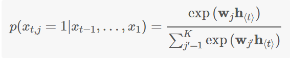
起初乍一看这个公式都会比较懵,但是很多论文中都会以这种形式来表示
S
o
f
t
M
a
x
SoftMax
SoftMax,这种写法实际上等价于
p
=
S
o
f
t
m
a
x
(
W
h
t
)
p=Softmax(Wh_{t})
p=Softmax(Wht)
解释一下,
W
j
W_{j}
Wj是参数矩阵W的第
j
j
j行,想一想,采用
S
o
f
t
M
a
x
SoftMax
SoftMax激活函数也就是输出
(
W
h
t
)
(Wh_{t})
(Wht)必须是一个向量所以
W
j
W_{j}
Wj与
h
t
h_{t}
ht作用产生了输出向量的第
j
j
j个维度,所以上面公式就可以理解了。
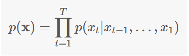
- 最后他用条件概率公式把每一个输出的条件概率相乘,得到了由输入到输出的一个概率,通过反响传播最大化这一分布:
R N N RNN RNN E n c o d e r − D e c o d e r Encoder-Decoder Encoder−Decoder
- 之前已经说过了,
R
N
N
RNN
RNN
E
n
c
o
d
e
r
−
D
e
c
o
d
e
r
Encoder-Decoder
Encoder−Decoder是把一个变长序列编码为一个定长向量表示,再把这个表示解码为另一个变长序列的过程。从概率论的角度看,这是学习两个变长序列之间的条件概率的方法:
p ( y 1 , . . . , y T ′ ∣ x 1 , . . . , x T ) p(y_{1},...,y_{T'}|x_{1},...,x_{T}) p(y1,...,yT′∣x1,...,xT)
Encoder
E
n
c
o
d
e
r
Encoder
Encoder是一个
R
N
N
,
RNN,
RNN,它顺序读入输入序列
X
X
X,并逐步更新隐状态(和普通的
R
N
N
RNN
RNN是一样的):
h
<
t
>
=
f
(
h
<
t
−
1
>
,
x
t
)
h_{<t>}=f(h_{<t-1>},x_{t})
h<t>=f(h<t−1>,xt)
读到序列结尾
(
E
O
S
)
(EOS)
(EOS)之后,
R
N
N
RNN
RNN的隐状态就是整个输入序列对应的表示
c
c
c。
Decoder
D
e
c
o
d
e
r
Decoder
Decoder也是一个
R
N
N
,
RNN,
RNN,这个
R
N
N
RNN
RNN的输入是
c
c
c,我们定义这个
R
N
N
RNN
RNN的隐藏层向量是
h
=
(
h
1
,
.
.
.
,
h
T
)
,
h=(h_{1},...,h_{T}),
h=(h1,...,hT),和之前的
R
N
N
RNN
RNN不同之处在于这个神经网络隐藏层向量h_{}的更新不仅取决于输入
c
c
c和前一个状态
h
<
t
−
1
>
h_{<t-1>}
h<t−1>,还取决于上一个输出
y
t
−
1
y_{t-1}
yt−1,这个设计的精妙之处就是重视了翻译中上下文之间语境的联系,公式如下:
h
<
t
>
=
f
(
h
<
t
−
1
>
,
c
,
y
t
−
1
)
h_{<t>}=f(h_{<t-1>},c,y_{t-1})
h<t>=f(h<t−1>,c,yt−1)
得到输出向量
y
y
y的思路大体上没有改变,得到条件分布仍然是采用
S
o
f
t
M
a
x
SoftMax
SoftMax
Encoder+Decoder
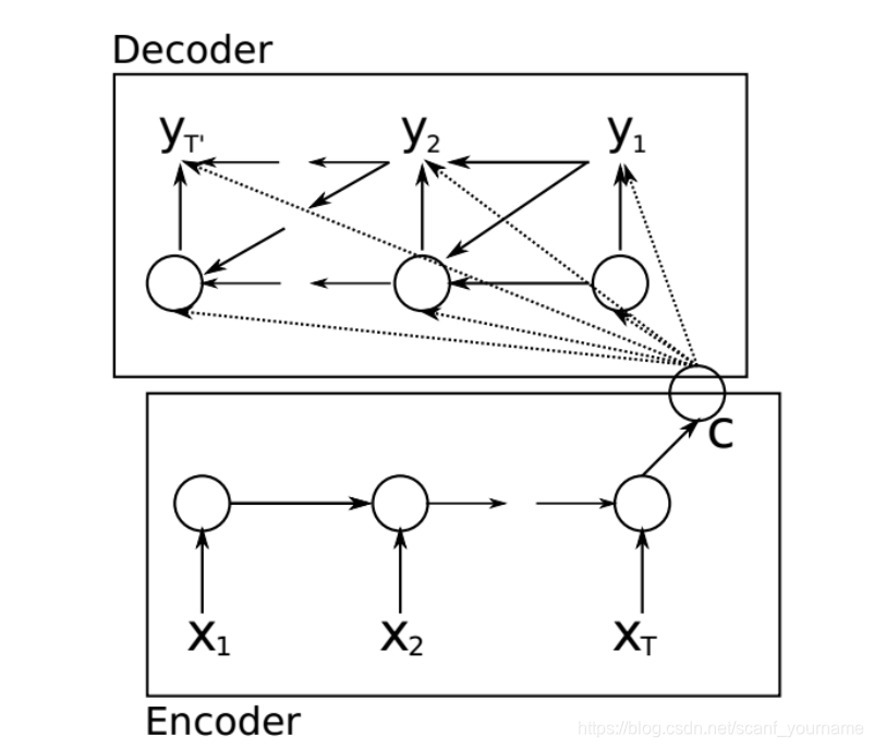
我们刚才所描述的步骤如上图所示,
E
n
c
o
d
e
r
Encoder
Encoder和
D
e
c
o
d
e
r
Decoder
Decoder共同进行训练,以最大化一个交叉熵损失函数: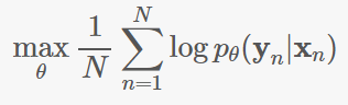
训练完
R
N
N
RNN
RNN
E
n
c
o
d
e
r
−
D
e
c
o
d
e
r
Encoder-Decoder
Encoder−Decoder之后,模型可以通过两种方式使用。一种是根据输入序列来生成输出序列。另一种是对给定的输入输出序列进行打分,分数就是概率
p
θ
(
y
n
∣
x
n
)
p_{\theta}(y_{n}|x_{n})
pθ(yn∣xn)
新的隐藏单元
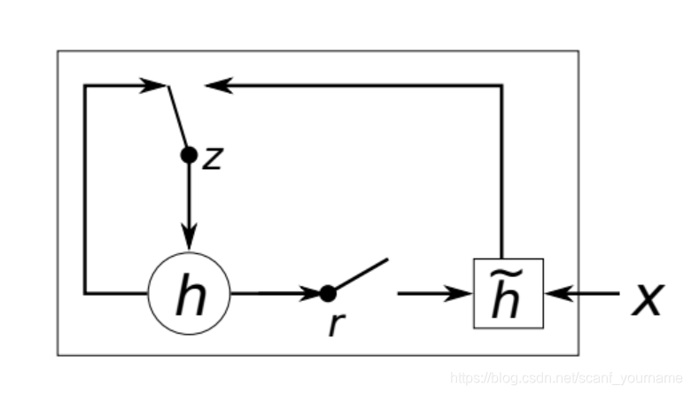
- 这一单元的灵感来自 L S T M , LSTM, LSTM,但是计算和实现都简单得多。图中 z z z是 u p d a t e update update g a t e , gate, gate,用于控制当前隐状态是否需要被新的隐状态 h ~ \widetilde{h} h 更新; r r r是 r e s e t reset reset g a t e , gate, gate,用于确定是否要丢弃上一个隐状态。
- 用一般的术语来说,下列内容实际上说明的是“一个
G
R
U
GRU
GRU
c
e
l
l
cell
cell中的一个
u
n
i
t
unit
unit的计算过程”,因此
r
j
r_{j}
rj、
z
j
z_{j}
zj和
h
j
<
t
>
h_{j}^{<t>}
hj<t>都是标量。
r j r_{j} rj的计算公式:
r j = σ ( [ W r x ] j + [ U r h < t − 1 > ] j ) r_{j}=\sigma([W_{r}x]_{j}+[U_{r}h_{<t-1>}]_{j}) rj=σ([Wrx]j+[Urh<t−1>]j)
其中 σ \sigma σ是 S i g m o i d Sigmoid Sigmoid激活函数, [ . ] j [.]_{j} [.]j是向量的第 j j j个元素, x x x是输入, h < t − 1 > h<t-1> h<t−1>是上一个隐藏状态, W r W_{r} Wr和 U r U_{r} Ur是学习到的权重矩阵
z j z_{j} zj的计算公式类似:
z j = σ ( [ W z x ] j + [ U z h < t − 1 > ] j ) z_{j}=\sigma([W_{z}x]_{j}+[U_{z}h_{<t-1>}]_{j}) zj=σ([Wzx]j+[Uzh<t−1>]j) - 单元
h
j
h_{j}
hj的实际激活状态通过下式计算:
h j < t > = z j h j < t − 1 > + ( 1 − z j ) h ~ < t > h_{j}^{<t>}=z_{j}h_{j}^{<t-1>}+(1-z_{j})\widetilde{h}^{<t>} hj<t>=zjhj<t−1>+(1−zj)h <t>
其中 h ~ < t > = ϕ ( [ W x ] j + [ U ( r ⨀ h < t − 1 > ) ] j ) \widetilde{h}^{<t>}=\phi([Wx]_{j}+[U(r \bigodot h_{<t-1>} )]_{j}) h <t>=ϕ([Wx]j+[U(r⨀h<t−1>)]j)
S M T SMT SMT模型和 R N N RNN RNN E n c o d e r − D e c o d e r Encoder-Decoder Encoder−Decoder的结合
- 传统的
S
M
T
SMT
SMT系统的目标是对于源句
e
,
e,
e,找到一个使下式最大化的翻译
f
f
f:
p ( f ∣ e ) ∝ p ( e ∣ f ) p ( f ) p(f|e)\propto p(e|f)p(f) p(f∣e)∝p(e∣f)p(f)
其中 p ( e ∣ f ) p(e|f) p(e∣f)称为翻译模型, p ( f ) p(f) p(f)称为语言模型。但在实际中,大部分 S M T SMT SMT系统都把 l o g p ( f ∣ e ) logp(f|e) logp(f∣e)做为一个log-linear模型,包括一些额外的feature和相应的权重:
l o g p ( f ∣ e ) = ∑ n = 1 N ω n f n ( f , e ) + l o g Z e logp(f|e)=\sum _{n=1}^{N}\omega _{n}f_{n}(f,e)+logZ_{e} logp(f∣e)=∑n=1Nωnfn(f,e)+logZe
其中 f n f_{n} fn是 f e a t u r e feature feature, ω n \omega _{n} ωn是权重, Z ( e ) Z(e) Z(e)是与权重无关的normalization constant。
在基于短语的 S M T SMT SMT模型中,翻译模型 p ( e ∣ f ) p(e|f) p(e∣f)被分解为源句和目标句中短语匹配的概率。这一概率再一次被作为 l o g − l i n e a r log-linear log−linear模型中的额外 f e a t u r e feature feature进行优化。 - 作者在一个短语对表中训练 R N N RNN RNN E n c o d e r − D e c o d e r , Encoder-Decoder, Encoder−Decoder,并将得到的分数作为 l o g − l i n e a r log-linear log−linear模型中的额外 f e a t u r e feature feature。目前的做法是把得到的短语对分数直接加入现有的短语对表中;事实上也可以直接用 R N N RNN RNN E n c o d e r − D e c o d e r Encoder-Decoder Encoder−Decoder代替这个表,但这就意味着对于每个源短语, R N N E n c o d e r − D e c o d e r RNN Encoder-Decoder RNNEncoder−Decoder都需要生成一系列好的目标短语,因此需要进行很多采样,这太昂贵了。
实验
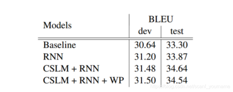
- 在 W M T ′ 14 WMT'14 WMT′14的 E n − F r En-Fr En−Fr任务上进行了评测。对于每种语言都只保留了最常见的 15000 15000 15000个词,将不常用的词标记为 [ U N K ] [UNK] [UNK]。
实验中, R N N E n c o d e r − D e c o d e r RNN Encoder-Decoder RNNEncoder−Decoder的 e n c o d e r encoder encoder和 d e c o d e r decoder decoder各有 1000 1000 1000个隐藏单元。每个输入符号 x < t > x_{<t>} x<t>和隐藏单元之间的输入矩阵用两个低秩 ( 100 ) (100) (100)矩阵来模拟,相当于学习了每个词的 100 100 100维 e m b e d d i n g embedding embedding。隐藏单元中的 h ~ \widetilde{h} h 使用的是双曲余弦函数 ( h y p e r b o l i c (hyperbolic (hyperbolic t a n g e n t tangent tangent f u n c t i o n ) function) function)。 d e c o d e r decoder decoder中隐状态到输出的计算使用的是一个深度神经网络,含有一个包含了 500 500 500个 m a x o u t maxout maxout单元的中间层。
R N N RNN RNN E n c o d e r − D e c o d e r Encoder-Decoder Encoder−Decoder的权重初值都是通过对一个各向同性的均值为零的高斯分布采样得到的,其标准差为 0.01 0.01 0.01。
通过
A
d
a
d
e
l
t
a
Adadelta
Adadelta和随机梯度下降法进行训练,其中超参数为
ϵ
=
1
0
−
6
\epsilon=10^{-6}
ϵ=10−6,
ρ
=
0.95
\rho =0.95
ρ=0.95.每次更新时,从短语表中随机选出
64
64
64个短语对。模型训练了大约
3
3
3天。
因为
C
S
L
M
CSLM
CSLM和
R
N
N
RNN
RNN
E
n
c
o
d
e
r
−
D
e
c
o
d
e
r
Encoder-Decoder
Encoder−Decoder共同使用能进一步提高表现,说明这两种方法对结果的贡献并不相同。
除此之外,它学习到的 w o r d word word e m b e d d i n g embedding embedding矩阵也是有意义的。
代码
import numpy as np
import torch
import torch.nn as nn
from torch.autograd import Variable

dtype = torch.FloatTensor
# S: Symbol that shows starting of decoding input
# E: Symbol that shows starting of decoding output
# P: Symbol that will fill in blank sequence if current batch data size is short than time steps

char_arr = [c for c in 'SEPabcdefghijklmnopqrstuvwxyz']
num_dic = {n: i for i, n in enumerate(char_arr)}

seq_data = [['man', 'women'], ['black', 'white'], ['king', 'queen'], ['girl', 'boy'], ['up', 'down'], ['high', 'low']]

# Seq2Seq Parameter
n_step = 5
n_hidden = 128
n_class = len(num_dic)
batch_size = len(seq_data)

def make_batch(seq_data):
    input_batch, output_batch, target_batch = [], [], []

    for seq in seq_data:
        for i in range(2):
            seq[i] = seq[i] + 'P' * (n_step - len(seq[i]))

        input = [num_dic[n] for n in seq[0]]
        output = [num_dic[n] for n in ('S' + seq[1])]
        target = [num_dic[n] for n in (seq[1] + 'E')]

        input_batch.append(np.eye(n_class)[input])
        output_batch.append(np.eye(n_class)[output])
        target_batch.append(target) # not one-hot

    # make tensor
    return Variable(torch.Tensor(input_batch)), Variable(torch.Tensor(output_batch)), Variable(torch.LongTensor(target_batch))

# Model
class Seq2Seq(nn.Module):
    def __init__(self):
        super(Seq2Seq, self).__init__()

        self.enc_cell = nn.RNN(input_size=n_class, hidden_size=n_hidden, dropout=0.5)
        self.dec_cell = nn.RNN(input_size=n_class, hidden_size=n_hidden, dropout=0.5)
        self.fc = nn.Linear(n_hidden, n_class)

    def forward(self, enc_input, enc_hidden, dec_input):
        enc_input = enc_input.transpose(0, 1) # enc_input: [max_len(=n_step, time step), batch_size, n_class]
        dec_input = dec_input.transpose(0, 1) # dec_input: [max_len(=n_step, time step), batch_size, n_class]

        # enc_states : [num_layers(=1) * num_directions(=1), batch_size, n_hidden]
        _, enc_states = self.enc_cell(enc_input, enc_hidden)
        # outputs : [max_len+1(=6), batch_size, num_directions(=1) * n_hidden(=128)]
        outputs, _ = self.dec_cell(dec_input, enc_states)

        model = self.fc(outputs) # model : [max_len+1(=6), batch_size, n_class]
        return model


input_batch, output_batch, target_batch = make_batch(seq_data)

model = Seq2Seq()
criterion = nn.CrossEntropyLoss()
optimizer = torch.optim.Adam(model.parameters(), lr=0.001)

for epoch in range(5000):
    # make hidden shape [num_layers * num_directions, batch_size, n_hidden]
    hidden = Variable(torch.zeros(1, batch_size, n_hidden))

    optimizer.zero_grad()
    # input_batch : [batch_size, max_len(=n_step, time step), n_class]
    # output_batch : [batch_size, max_len+1(=n_step, time step) (becase of 'S' or 'E'), n_class]
    # target_batch : [batch_size, max_len+1(=n_step, time step)], not one-hot
    output = model(input_batch, hidden, output_batch)
    # output : [max_len+1, batch_size, num_directions(=1) * n_hidden]
    output = output.transpose(0, 1) # [batch_size, max_len+1(=6), num_directions(=1) * n_hidden]
    loss = 0
    for i in range(0, len(target_batch)):
        # output[i] : [max_len+1, num_directions(=1) * n_hidden, target_batch[i] : max_len+1]
        loss += criterion(output[i], target_batch[i])
    if (epoch + 1) % 1000 == 0:
        print('Epoch:', '%04d' % (epoch + 1), 'cost =', '{:.6f}'.format(loss))
    loss.backward()
    optimizer.step()


# Test
def translate(word):
    input_batch, output_batch, _ = make_batch([[word, 'P' * len(word)]])

    # make hidden shape [num_layers * num_directions, batch_size, n_hidden]
    hidden = Variable(torch.zeros(1, 1, n_hidden))
    output = model(input_batch, hidden, output_batch)
    # output : [max_len+1(=6), batch_size(=1), n_class]

    predict = output.data.max(2, keepdim=True)[1] # select n_class dimension
    decoded = [char_arr[i] for i in predict]
    end = decoded.index('E')
    translated = ''.join(decoded[:end])

    return translated.replace('P', '')

print('test')
print('man ->', translate('man'))
print('mans ->', translate('mans'))
print('king ->', translate('king'))
print('black ->', translate('black'))
print('upp ->', translate('upp'))


 888
888

 被折叠的 条评论
为什么被折叠?
被折叠的 条评论
为什么被折叠?
 到【灌水乐园】发言


