组队学习第二天：心跳信号分类之baseline学习

原题目地址：零基础入门数据挖掘-心跳信号分类预测
本文是鸣鹤星空小组组队学习的集体成果。
id:李由，一只小呆

1 EDA 目标

• EDA的价值主要在于熟悉数据集，了解数据集，对数据集进行验证来确定所获得数据集可以用于接下来的机器学习或者深度学习使用。
• 当了解了数据集之后我们下一步就是要去了解变量间的相互关系以及变量与预测值之间的存在关系。
• 引导数据科学从业者进行数据处理以及特征工程的步骤,使数据集的结构和特征集让接下来的预测问题更加可靠。
• 完成对于数据的探索性分析，并对于数据进行一些图表或者文字总结并打卡。

2 内容介绍

2.1 载入各种数据科学以及可视化库:

• 数据科学库 pandas、numpy、scipy；
• 可视化库 matplotlib、seabon；

2.2载入数据：

• 载入训练集和测试集；
• 简略观察数据(head()+shape)；

2.3数据总览:

• 通过describe()来熟悉数据的相关统计量
• 通过info()来熟悉数据类型

2.4判断数据缺失和异常：

• 查看每列的存在nan情况
• 异常值检测

2.5了解预测值的分布

• 总体分布概况
• 查看skewness and kurtosis
• 查看预测值的具体频数

3 代码和运行截图

1.载入各种数据科学与可视化库

#coding:utf-8

import warnings
warnings.filterwarnings('ignore')
import missingno as msno
import pandas as pd
from pandas import DataFrame,Series
import matplotlib.pyplot as plt
import seaborn as sns
import numpy as np

2.载入训练集和测试集

Train_data = pd.read_csv('./data/train.csv')
Test_data = pd.read_csv('./data/testA.csv')

3.观察训练集和测试集首尾数据

Train_data.head().append(Train_data.tail())

	id	heartbeat_signals	label
0	0	0.9912297987616655,0.9435330436439665,0.764677...	0.0
1	1	0.9714822034884503,0.9289687459588268,0.572932...	0.0
2	2	1.0,0.9591487564065292,0.7013782792997189,0.23...	2.0
3	3	0.9757952826275774,0.9340884687738161,0.659636...	0.0
4	4	0.0,0.055816398940721094,0.26129357194994196,0...	2.0
99995	99995	1.0,0.677705342021188,0.22239242747868546,0.25...	0.0
99996	99996	0.9268571578157265,0.9063471198026871,0.636993...	2.0
99997	99997	0.9258351628306013,0.5873839035878395,0.633226...	3.0
99998	99998	1.0,0.9947621698382489,0.8297017704865509,0.45...	2.0
99999	99999	0.9259994004527861,0.916476635326053,0.4042900...	0.0

Train_data.shape

(100000, 3)

Test_data.head().append(Test_data.tail())

	id	heartbeat_signals
0	100000	0.9915713654170097,1.0,0.6318163407681274,0.13...
1	100001	0.6075533139615096,0.5417083883163654,0.340694...
2	100002	0.9752726292239277,0.6710965234906665,0.686758...
3	100003	0.9956348033996116,0.9170249621481004,0.521096...
4	100004	1.0,0.8879490481178918,0.745564725322326,0.531...
19995	119995	1.0,0.8330283177934747,0.6340472606311671,0.63...
19996	119996	1.0,0.8259705825857048,0.4521053488322387,0.08...
19997	119997	0.951744840752379,0.9162611283848351,0.6675251...
19998	119998	0.9276692903808186,0.6771898159607004,0.242906...
19999	119999	0.6653212231837624,0.527064114047737,0.5166625...

Test_data.shape

(20000, 2)

Train_data.describe()

	id	label
count	100000.000000	100000.000000
mean	49999.500000	0.856960
std	28867.657797	1.217084
min	0.000000	0.000000
25%	24999.750000	0.000000
50%	49999.500000	0.000000
75%	74999.250000	2.000000
max	99999.000000	3.000000

Train_data.info()

<class 'pandas.core.frame.DataFrame'>
RangeIndex: 100000 entries, 0 to 99999
Data columns (total 3 columns):
 #   Column             Non-Null Count   Dtype  
---  ------             --------------   -----  
 0   id                 100000 non-null  int64  
 1   heartbeat_signals  100000 non-null  object 
 2   label              100000 non-null  float64
dtypes: float64(1), int64(1), object(1)
memory usage: 2.3+ MB

Test_data.describe()

	id
count	20000.000000
mean	109999.500000
std	5773.647028
min	100000.000000
25%	104999.750000
50%	109999.500000
75%	114999.250000
max	119999.000000

Test_data.info()

<class 'pandas.core.frame.DataFrame'>
RangeIndex: 20000 entries, 0 to 19999
Data columns (total 2 columns):
 #   Column             Non-Null Count  Dtype 
---  ------             --------------  ----- 
 0   id                 20000 non-null  int64 
 1   heartbeat_signals  20000 non-null  object
dtypes: int64(1), object(1)
memory usage: 312.6+ KB

4.判断数据缺失和异常

Train_data.isnull().sum()

id                   0
heartbeat_signals    0
label                0
dtype: int64

Test_data.isnull().sum()

id                   0
heartbeat_signals    0
dtype: int64

Train_data['label']

0        0.0
1        0.0
2        2.0
3        0.0
4        2.0
        ... 
99995    0.0
99996    2.0
99997    3.0
99998    2.0
99999    0.0
Name: label, Length: 100000, dtype: float64

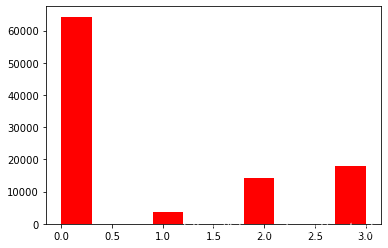
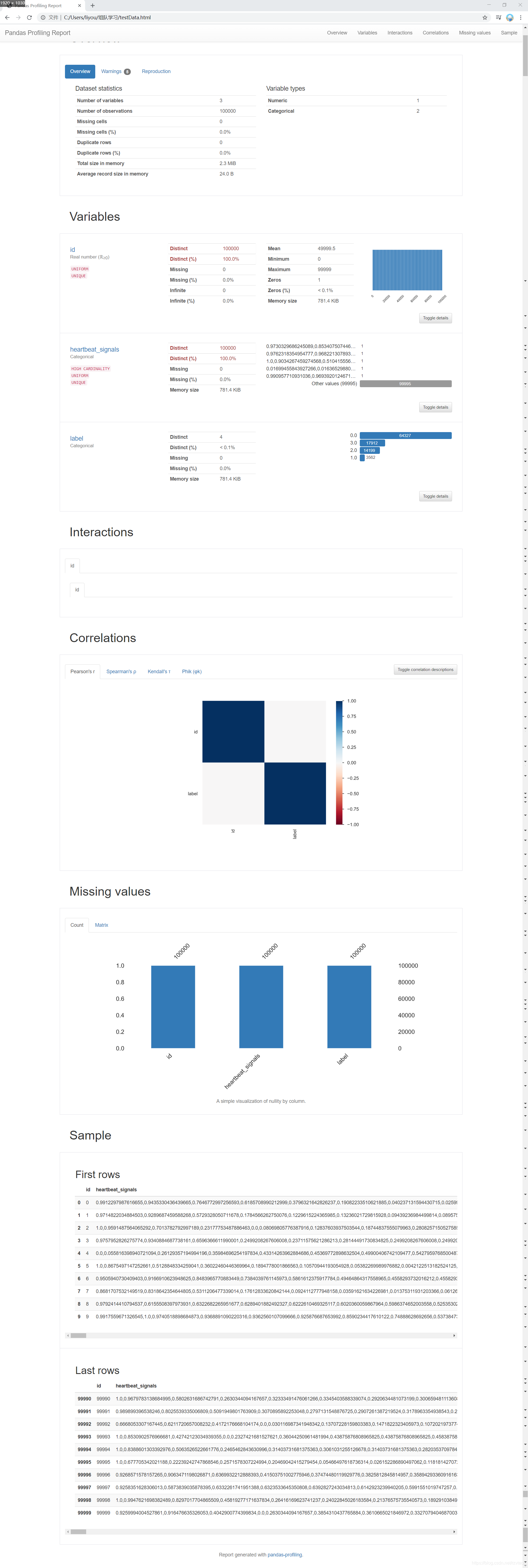
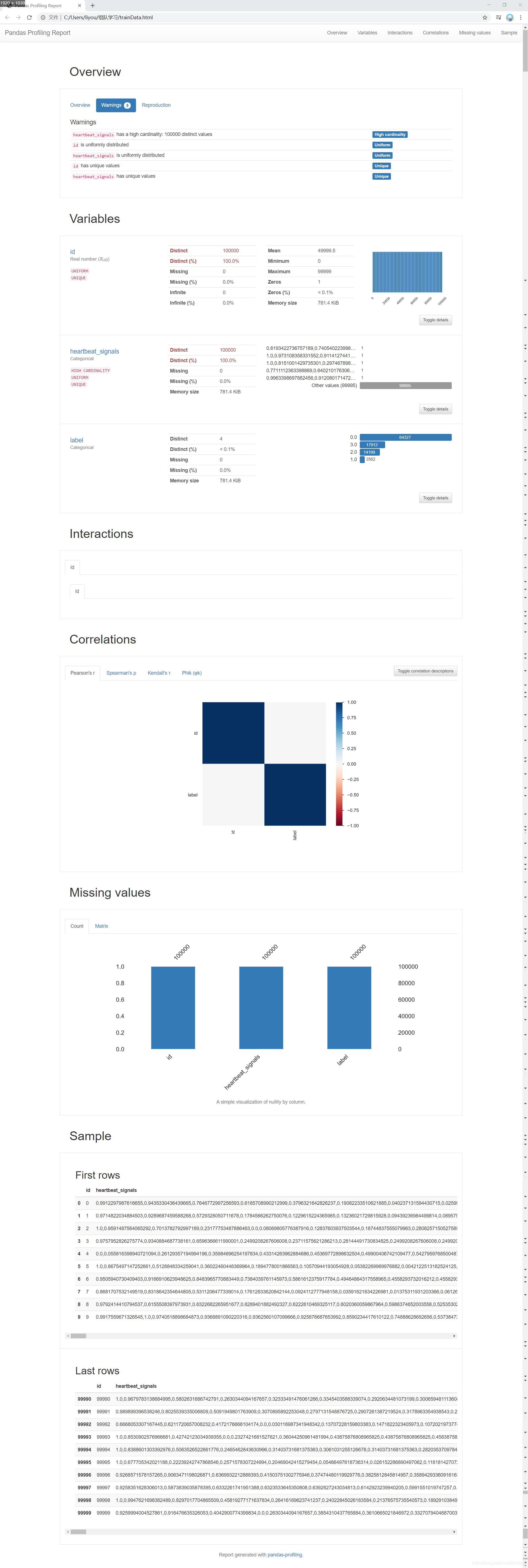
Train_data['label'].value_counts()

0.0    64327
3.0    17912
2.0    14199
1.0     3562
Name: label, dtype: int64

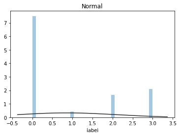
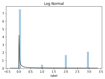
1)有界分布情况（无界约翰逊分布等）

import scipy.stats as st
y = Train_data['label']
plt.figure(1);plt.title('Default')
sns.distplot(y, rug = True, bins = 20)
plt.figure(2);plt.title('Normal')
sns.distplot(y, kde = False, fit = st.norm)
plt.figure(3);plt.title('Log Normal')
sns.distplot(y, kde = False, fit = st.lognorm)

<matplotlib.axes._subplots.AxesSubplot at 0x13b375faf10>

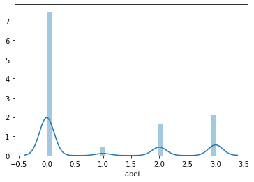
2)查看skewness和kurtosis

sns.distplot(Train_data['label']);
print("Skewness: %f" % Train_data['label'].skew())
print("Kurtosis: %f" % Train_data['label'].kurt())

Skewness: 0.871005
Kurtosis: -1.009573

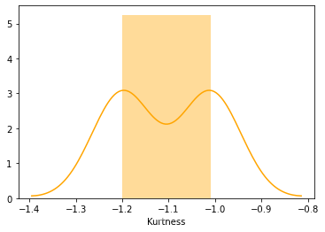
Train_data.skew(), Train_data.kurt()

(id       0.000000
 label    0.871005
 dtype: float64,
 id      -1.200000
 label   -1.009573
 dtype: float64)

sns.distplot(Train_data.kurt(),color='orange',axlabel='Kurtness')

<matplotlib.axes._subplots.AxesSubplot at 0x13b38833cd0>

3）查看预测值的具体频数

plt.hist(Train_data['label'], orientation= 'vertical', histtype= 'bar', color='red')
plt.show()

import pandas_profiling

pfr = pandas_profiling.ProfileReport(Train_data)
pfr.to_file("./trainData.html")
pfr1 = pandas_profiling.ProfileReport(Test_data)
pfr.to_file("./testData.html")

Summarize dataset:   0%|          | 0/16 [00:00<?, ?it/s]



Generate report structure:   0%|          | 0/1 [00:00<?, ?it/s]



Render HTML:   0%|          | 0/1 [00:00<?, ?it/s]



Export report to file:   0%|          | 0/1 [00:00<?, ?it/s]



Export report to file:   0%|          | 0/1 [00:00<?, ?it/s]


Generate report structure:   0%|          | 0/1 [00:00<?, ?it/s]



Render HTML:   0%|          | 0/1 [00:00<?, ?it/s]



Export report to file:   0%|          | 0/1 [00:00<?, ?it/s]



Export report to file:   0%|          | 0/1 [00:00<?, ?it/s]

4 感想

通过数据探索性分析，我们对数据的各个统计量有了清楚直观的了解。这为我们对其进行下一步分析奠定了坚实基础。
数据分析时可以使用很多功能强大的库，使我们的操作事半功倍。